SpaPheno Tutorial: Linking Spatial Transcriptomics to Clinical Phenotypes with Interpretable Machine Learning

Introduction

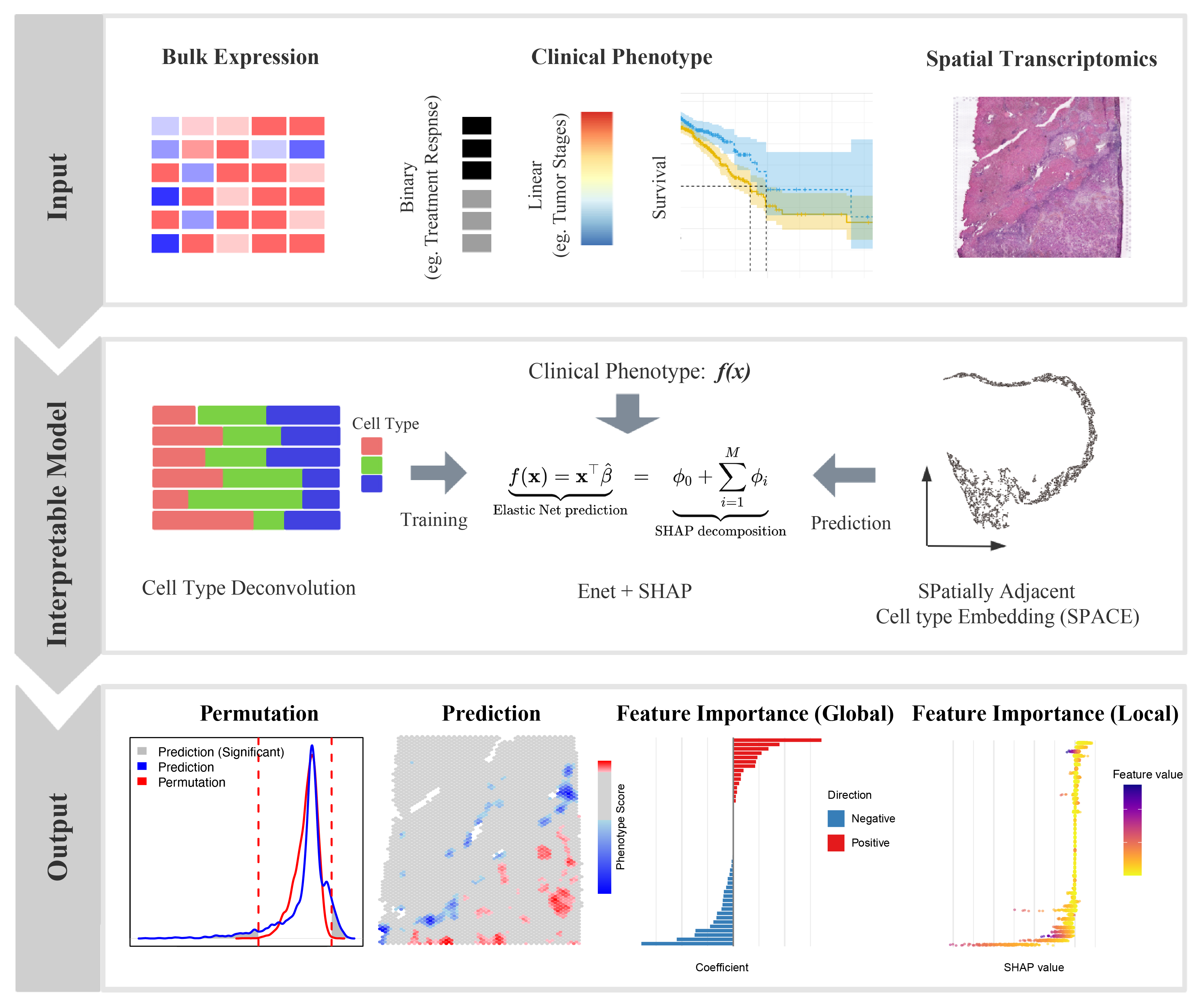
Linking spatial transcriptomic patterns to clinically relevant phenotypes is a critical step toward spatially informed precision oncology. Here, we introduce SpaPheno, an interpretable machine learning framework that integrates spatial transcriptomics with clinically annotated bulk RNA-seq data to uncover spatially resolved biomarkers predictive of patient outcomes. Leveraging Elastic Net regression combined with SHAP-based attribution, SpaPheno uniquely identifies spatial features at multiple scales—from tissue regions to specific cell types and individual spatial spots—that are associated with patient survival, tumor stage, and immunotherapy response. We demonstrate the robustness and generalizability of SpaPheno through comprehensive simulations and applications spanning primary liver cancer, clear cell renal cell carcinoma, breast cancer, and melanoma. Across these diverse settings, SpaPheno achieves high predictive accuracy while providing biologically meaningful and spatially precise interpretations. Our framework offers a powerful and extensible approach for translating complex spatial omics data into actionable clinical insights, accelerating the development of precision oncology strategies grounded in tumor spatial architecture.

Here are Key Features of SpaPheno:

Integration of spatial transcriptomics with clinically annotated bulk RNA-seq data
Multi-scale interpretable machine learning framework
Robust applicability across diverse cancer types and clinical endpoints

The Overview of SpaPheno

Installation

To get started with SpaPheno, ensure that you have the required dependencies installed. The package relies on a set of CRAN and Bioconductor packages such as glmnet, FNN, and survival. You can install them via BiocManager if not already available.

Next, install SpaPheno directly from GitHub using devtools. This will fetch the latest development version maintained by the authors.

Once installed, load the core packages used throughout the SpaPheno workflow, including ggplot2 for visualization and tidyverse for data handling.

if (!require("BiocManager", quietly = TRUE)) {
  install.packages("BiocManager")
}

## Install suggested packages
# BiocManager::install(c(
#   "glmnet",
#   "FNN",
#   "survival"
# ))

# install.packages("devtools")
# devtools::install_github("bm2-lab/SpaDo")

# SpaPheno installation
# devtools::install_github("Duan-Lab1/SpaPheno", dependencies = c("Depends", "Imports", "LinkingTo"))
# install.packages("SpaPheno_0.0.2.tar.gz", repos = NULL, type = "source")

library(SpaPheno)
library(tidyverse)
library(ggplot2)
library(reshape2)
library(stringr)
library(survival)

Data availability

The data required for the test are all listed in the following google cloud directory SpaPheno Demo Data.

├── BRCAsurvival.RData
├── HCC_stage.RData
├── HCC_survival.RData
├── KIRC_survival.RData
├── Melanoma_ICB.RData
├── Simulation_osmFISH.RData
└── Simulation_STARmap.RData

In addition to the demonstration datasets above, we provide standardized pan-cancer bulk and single-cell reference resources to support cross-cohort and multi-omic applications of SpaPheno SpaPheno TCGA-scRNARef-Dataset:

No.	TCGA Standard Cancer Type	Corresponding Single-Cell Data Original Naming
1	BLCA	BLCA
2	BRCA	BRCA / Breast
3	CESC	CESC
4	CHOL	CHOL
5	COAD	CRC
6	ESCA	ESCA
7	HNSC	HNSC / HNSCC / Oral
8	KICH	KICH
9	KIRC	KIRC
10	LIHC	LIHC / Liver
11	LUAD	LUAD
12	LUSC	LSCC
13	OV	OV / Ovary
14	PAAD	PAAD
15	PRAD	PRAD
16	SKCM	SKCM
17	STAD	STAD
18	THCA	THCA
19	UCEC	UCEC
20	UVM	UVM

TCGA Pan-Cancer Bulk Expression and Clinical Data:

Processed RNA-seq gene expression profiles (raw counts) and corresponding clinical annotations (including survival outcomes, tumor stage) for 20 common cancer types from The Cancer Genome Atlas (TCGA) are available. The included cancer types are listed in the table below, with unified gene symbols and standardized phenotype annotations to facilitate direct use with SpaPheno:

TCGA-n20PanCaner_Dataset
├── TCGA-BLCA
│   ├── BLCA_summary.csv
│   ├── BLCA_expression_by_gene_name.tsv
│   ├── BLCA_expression.tsv
│   ├── BLCA_phenotype_with_survival.csv
│   └── BLCA_phenotype.csv
├── TCGA-BRCA
├── TCGA-CESC
├── TCGA-CHOL
├── TCGA-COAD
├── TCGA-ESCA
├── TCGA-HNSC
├── TCGA-KICH
├── TCGA-KIRC
├── TCGA-LIHC
├── TCGA-LUAD
├── TCGA-LUSC
├── TCGA-OV
├── TCGA-PAAD
├── TCGA-PRAD
├── TCGA-SKCM
├── TCGA-STAD
├── TCGA-THCA
├── TCGA-UCEC
└── TCGA-UVM

TabulaTIME Single-Cell Reference Data:

Matched single-cell RNA-seq reference datasets for the above cancer types, derived from the TabulaTIME database, are provided as preprocessed Seurat objects. These datasets include cell type annotations, enabling direct integration with spatial transcriptomics data for cell type deconvolution and spatially resolved interpretation in SpaPheno.

TabulaTIME_scRNA_ref/
├── TabulaTIME_reference_summary.csv
├── BLCA_ref.rds
├── BRCA_ref.rds
├── CESC_ref.rds
├── CHOL_ref.rds
├── CRC-COAD_ref.rds
├── ESCA_ref.rds
├── HNSC_ref.rds
├── KICH_ref.rds
├── KIRC_ref.rds
├── LIHC_ref.rds
├── LSCC-LUSC_ref.rds
├── LUAD_ref.rds
├── OV_ref.rds
├── PAAD_ref.rds
├── PRAD_ref.rds
├── SKCM_ref.rds
├── STAD_ref.rds
├── THCA_ref.rds
├── UCEC_ref.rds
└── UVM_ref.rds

Deconvolution Strategy

To enable consistent and comparable phenotype association analysis across data types, SpaPheno performs cell-type deconvolution on both bulk RNA-seq and spatial transcriptomics (ST) data using a shared single-cell RNA-seq reference dataset.

In the current implementation, cell2location is used to estimate cell-type abundance profiles, ensuring that downstream phenotype modeling is built on unified, biologically interpretable features.

Parameter Selection for cell2location

When performing deconvolution with cell2location, two key parameters should be carefully adjusted based on the input data modality:

1. N_cells_per_location

This parameter specifies the expected number of cells contributing to each measured profile.

Spatial transcriptomics (e.g., 10x Visium)

Each spot captures a mixture of multiple cells.

A reasonable range is:

N_cells_per_location = 10–30

Default setting in SpaPheno:

N_cells_per_location = 20

Bulk RNA-seq

Each sample represents a large aggregate of cells.

Following cell2location recommendations, a moderate-to-large value is used:

N_cells_per_location = 1–100

Default setting in SpaPheno:

N_cells_per_location = 100

2. detection_alpha

This parameter controls regularization strength for per-sample normalization, accounting for technical variation in RNA detection efficiency.

Lower values (e.g., 20)

→ Stronger normalization and adaptation to technical noise

→ More suitable for spatial transcriptomics, which typically exhibits higher technical heterogeneity

Higher values (e.g., 200)

→ Weaker normalization, assuming more stable detection sensitivity

→ More suitable for bulk RNA-seq, where technical variation is relatively modest

Default settings used in SpaPheno:

Visium spatial transcriptomics: detection_alpha = 20

Bulk RNA-seq: detection_alpha = 200

Practical Recommendations

Parameter choice should reflect both biological structure and technical characteristics:

Spot-based spatial data

→ Use relatively low N_cells_per_location

→ Use moderate or low detection_alpha

Bulk or bulk-like profiling data

→ Use higher N_cells_per_location

→ Use higher detection_alpha

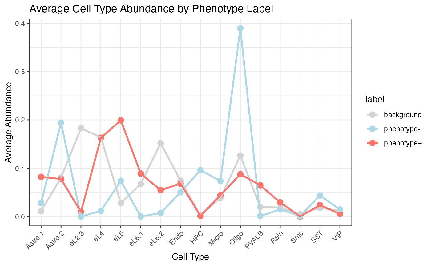
Simulation osmFISH

This tutorial demonstrates the workflow of SpaPheno using simulated osmFISH data, including:

Loading and visualizing spatial cell annotations.
Defining simulated phenotypes across spatial regions.
Generating pseudo-bulk samples for phenotype modeling.
Building a logistic regression model via automated regularization selection.
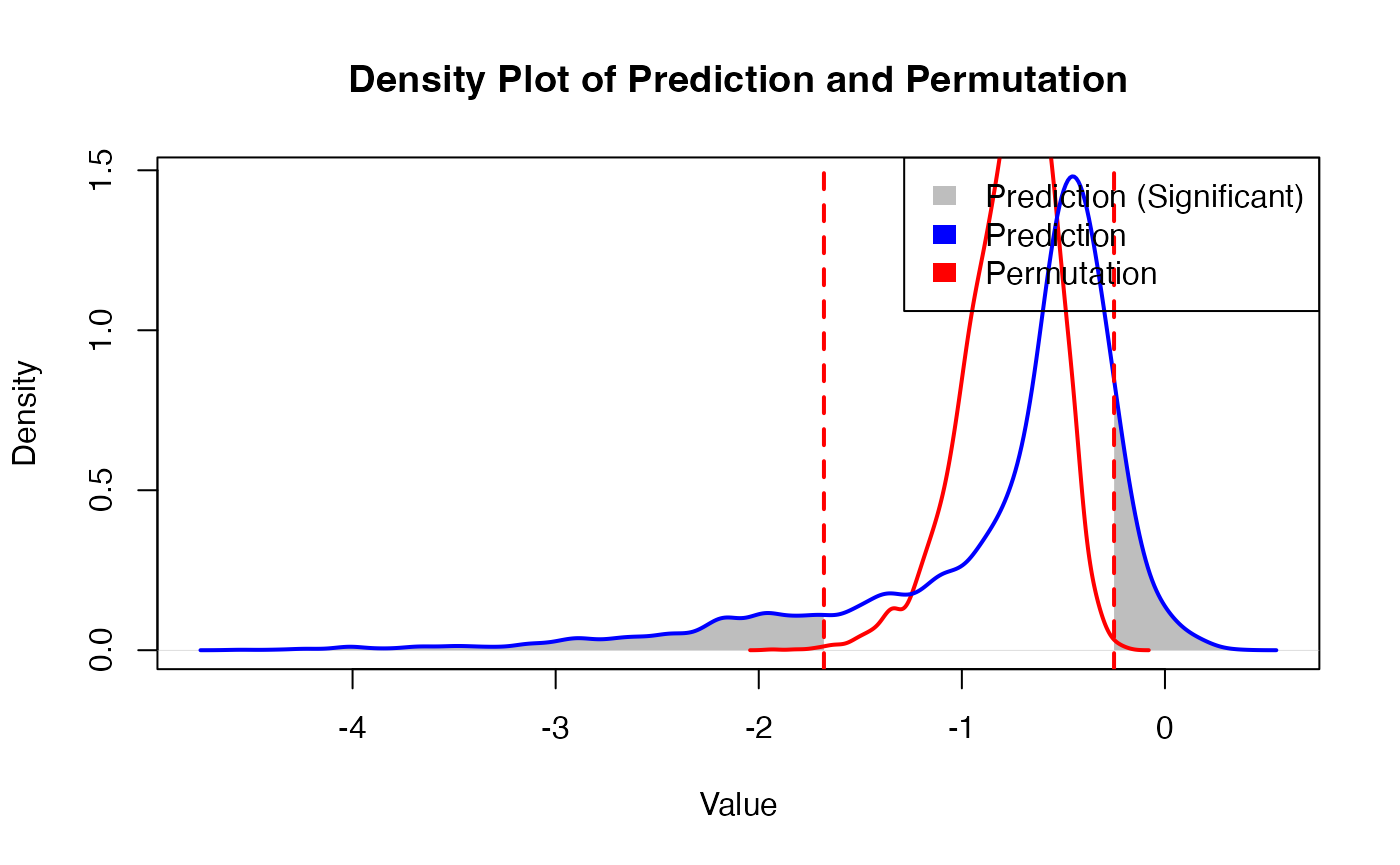
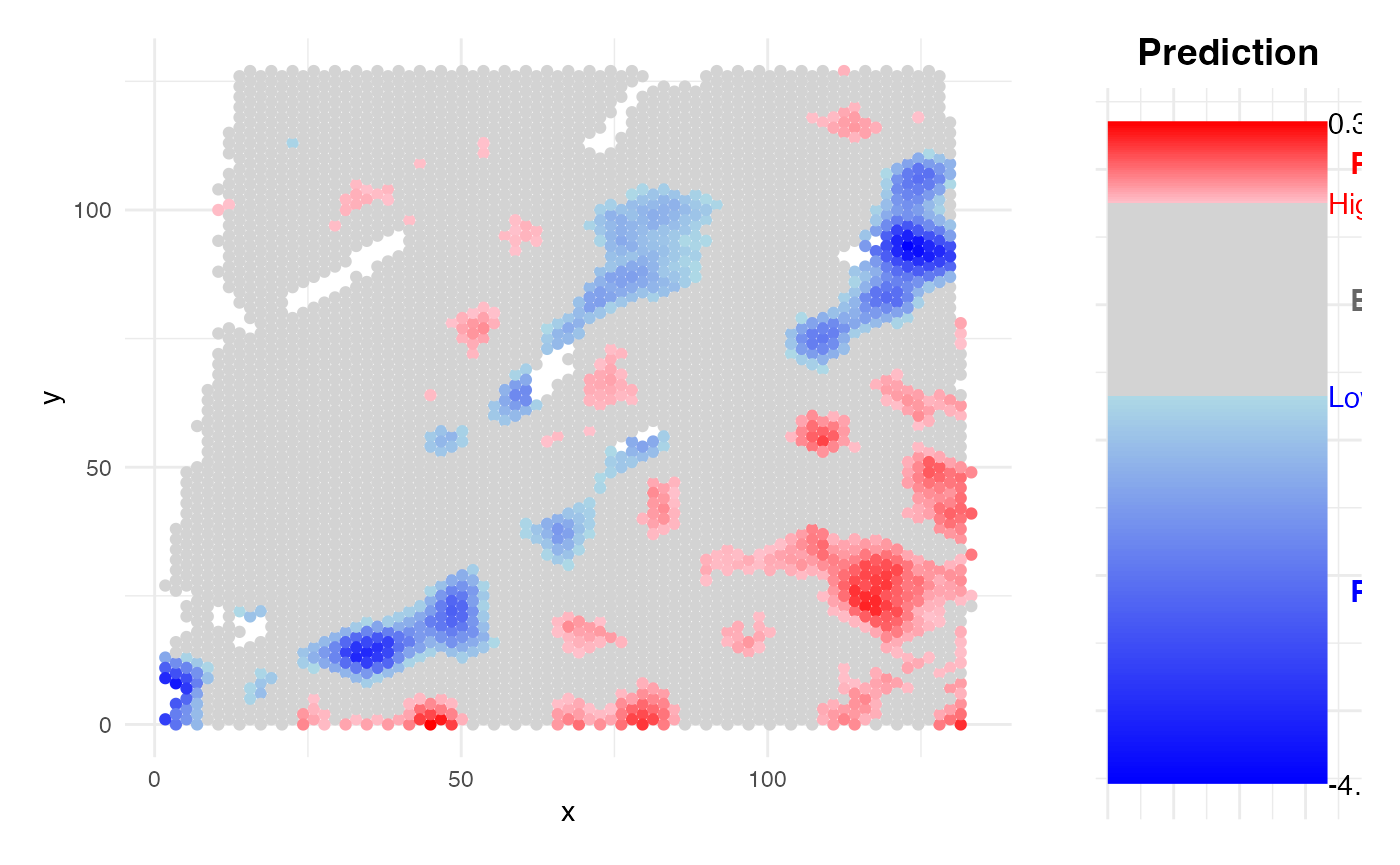
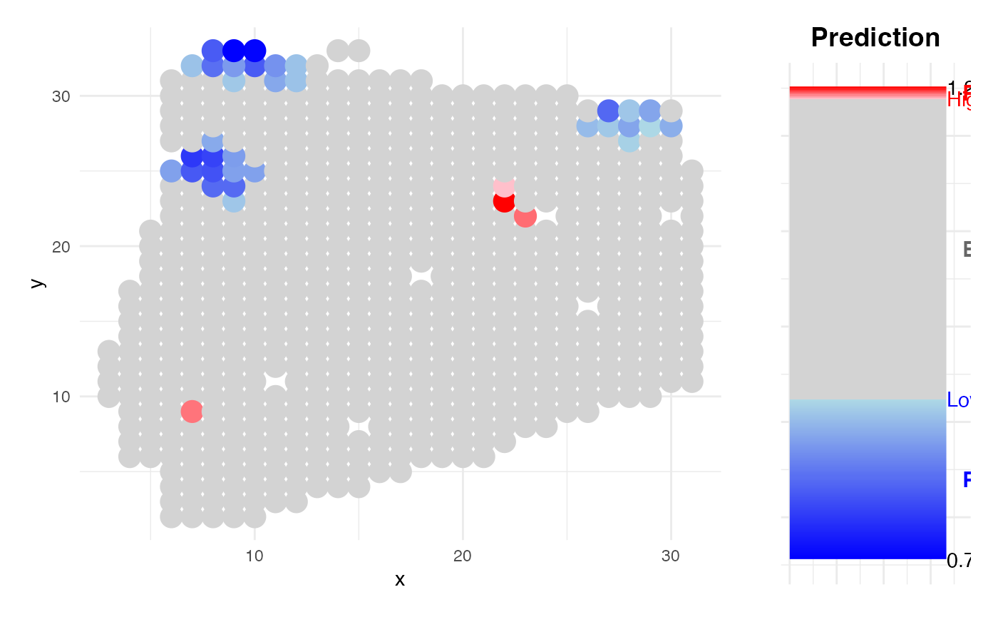
Performing spatial phenotype risk prediction.
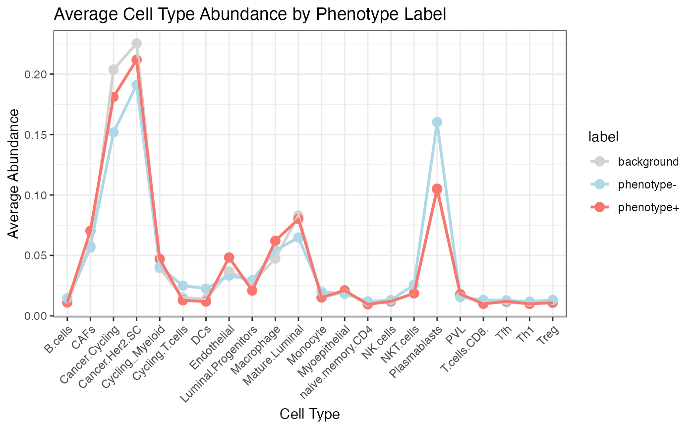
Interpreting key contributing cell types using SHAP values.
Exploring spatial patterns of model residuals for biological insight.

Together, this pipeline allows researchers to integrate spatial structure, cell composition, and predictive modeling to understand how local cell-type environments contribute to complex phenotypes.

load data

rm(list = ls())

load(system.file("extdata", "Simulation_osmFISH.RData", package = "SpaPheno"))

ggplot(test_coordinate, aes(x = X, y = Y, color = sample_information_cellType)) +
  geom_point(size = 1)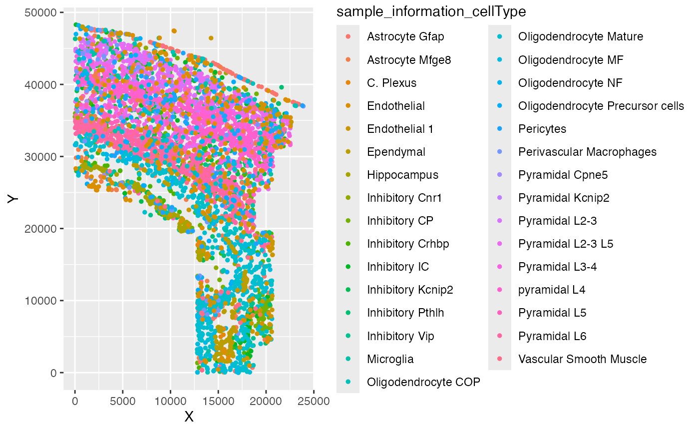

ggplot(test_coordinate, aes(x = X, y = Y, color = sample_information_region)) +
  geom_point(size = 1)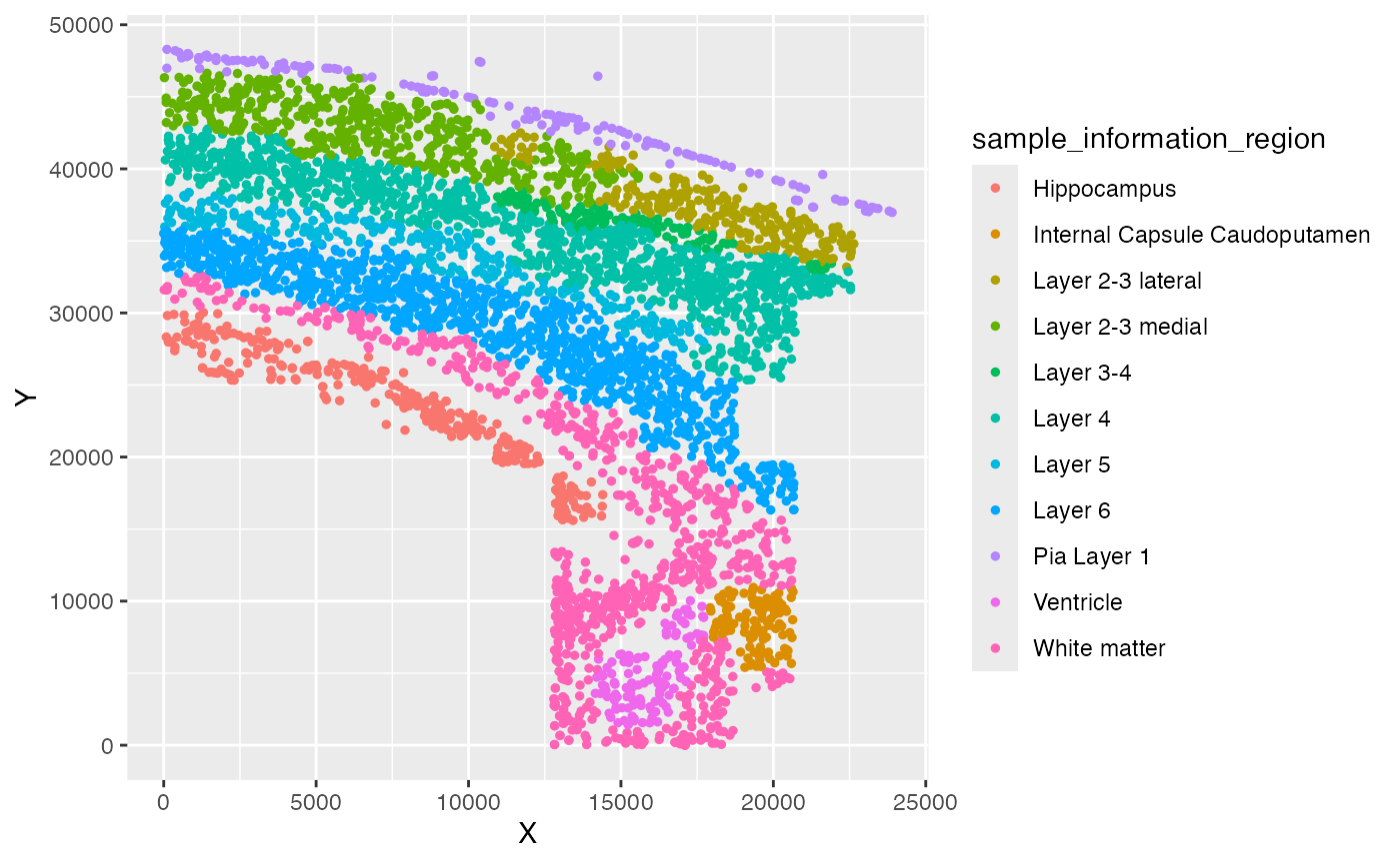

Choose simulated phenotypes

region_all <- names(table(sample_information_region))
phenotype_simu <- region_all[c(3, 4)]
sample_information_region_choose <- sample_information_region
sample_information_region_choose[!sample_information_region_choose %in% phenotype_simu] <- NA

Ground truth of simulated phenotypes

custom_colors <- c("red", "lightgray", "blue")
names(custom_colors) <- c(phenotype_simu[2], "Background", phenotype_simu[1])
sample_information_region_choose[!sample_information_region_choose %in% phenotype_simu] <- "Background"
Ground_truth <- factor(sample_information_region_choose[row.names(test_coordinate)], levels = c(phenotype_simu[1], "Background", phenotype_simu[2]))
ggplot(test_coordinate, aes(x = X, y = Y, color = Ground_truth)) +
  geom_point(size = 1) +
  scale_color_manual(values = custom_colors)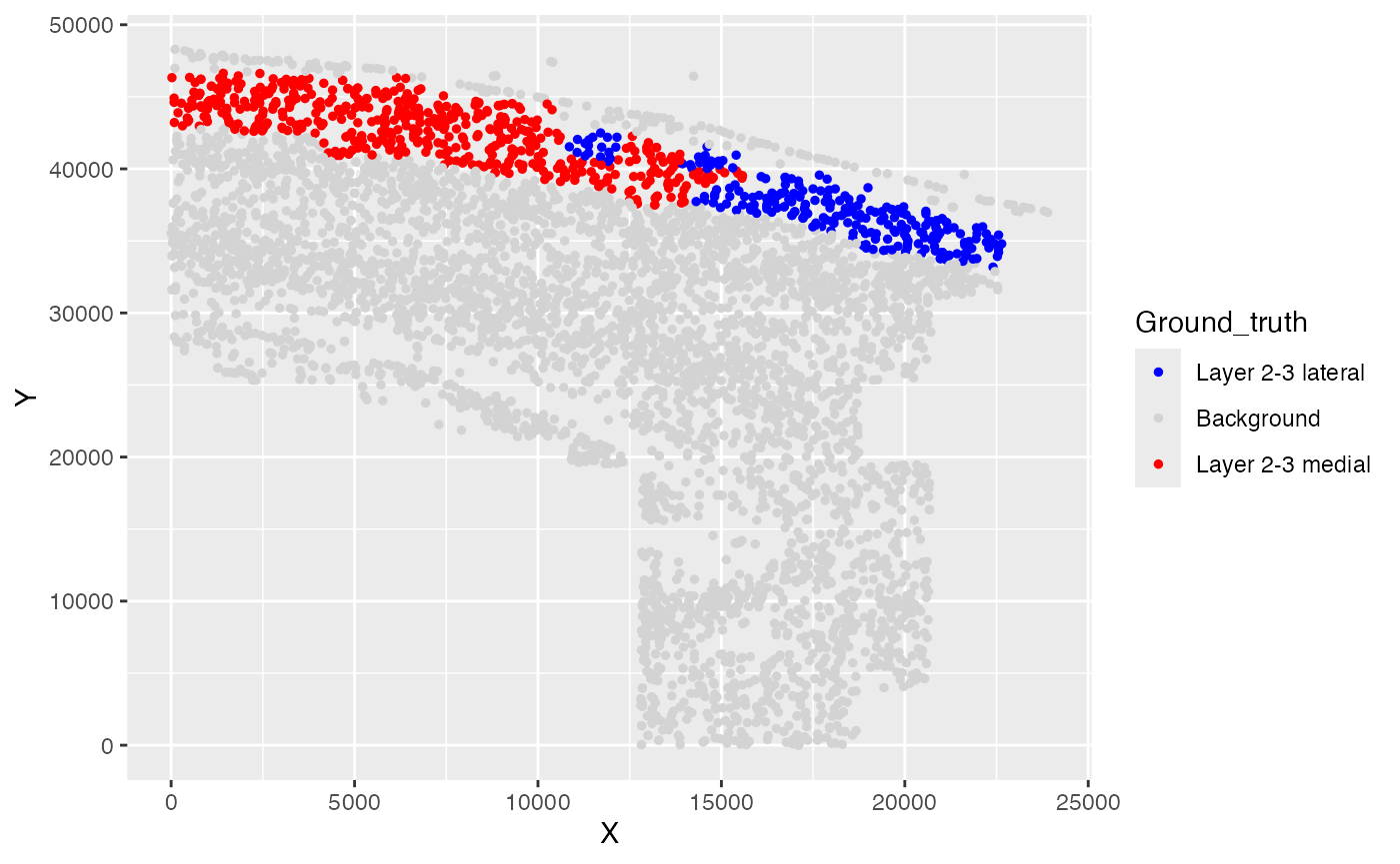

Simulating bulk data with phenotypes

pseudo_bulk_simi <- generate_simulated_bulk_data(
  input_data = sample_information_cellType, 
  region_labels = sample_information_region, 
  phenotypes = phenotype_simu, 
  perturbation_percent = 0.1, 
  num_samples = 50, 
  mode = "proportion")

pseudo_bulk_df1 <- pseudo_bulk_simi[[1]]
pseudo_bulk_df2 <- pseudo_bulk_simi[[2]]

bulk_decon <- t(as.matrix(cbind(pseudo_bulk_df1, pseudo_bulk_df2)))
bulk_pheno <- rep(c(0, 1), each = 50)
names(bulk_pheno) <- c(colnames(pseudo_bulk_df1), colnames(pseudo_bulk_df2))
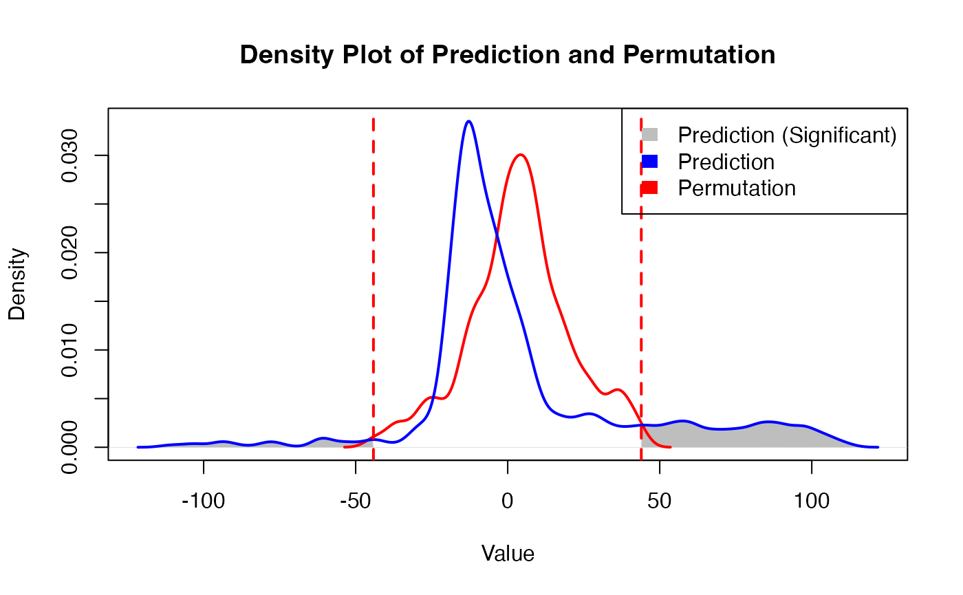
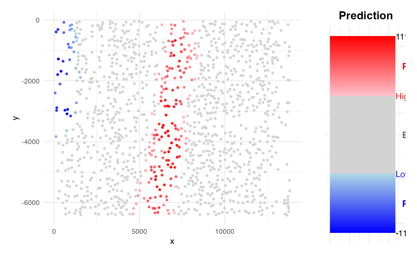
family <- "binomial"

Obtaining prediction results

PhenoResult <- SpatialPhenoMap(
  bulk_decon = bulk_decon, 
  bulk_pheno = bulk_pheno, 
  family = family, 
  coord = test_coordinate, 
  resolution = "single_cell", 
  sample_information_cellType = sample_information_cellType, 
  n_perm = 1, 
  p = 0.001)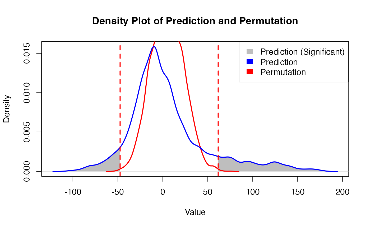

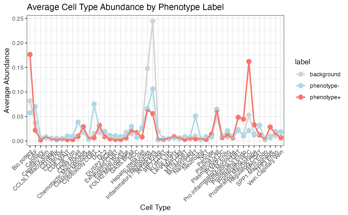
SHAP analysis

pred_result <- PhenoResult$pred_score
phenoPlus <- row.names(pred_result[pred_result$label %in% "phenotype+", ])

model <- PhenoResult$model
X <- as.data.frame(PhenoResult$cell_type_distribution[phenoPlus, ])

## This step took a very long time
# shap_test_plus <- compute_shap_spatial(
#   model = model, 
#   X_bulk = as.data.frame(bulk_decon), 
#   y_bulk = bulk_pheno, 
#   X_spatial = X)

head(shap_test_plus)

##           feature           phi      phi.var feature.value    sample
## 1  Astrocyte.Gfap  0.0000000000 0.000000e+00          0.08 cell_5682
## 2 Astrocyte.Mfge8  0.0000000000 0.000000e+00          0.04 cell_5682
## 3       C..Plexus -0.0134631352 4.616196e-03          0.02 cell_5682
## 4     Endothelial  0.0000000000 0.000000e+00          0.06 cell_5682
## 5   Endothelial.1  0.0002035102 1.812159e-05          0.02 cell_5682
## 6       Ependymal  0.0000000000 0.000000e+00          0.00 cell_5682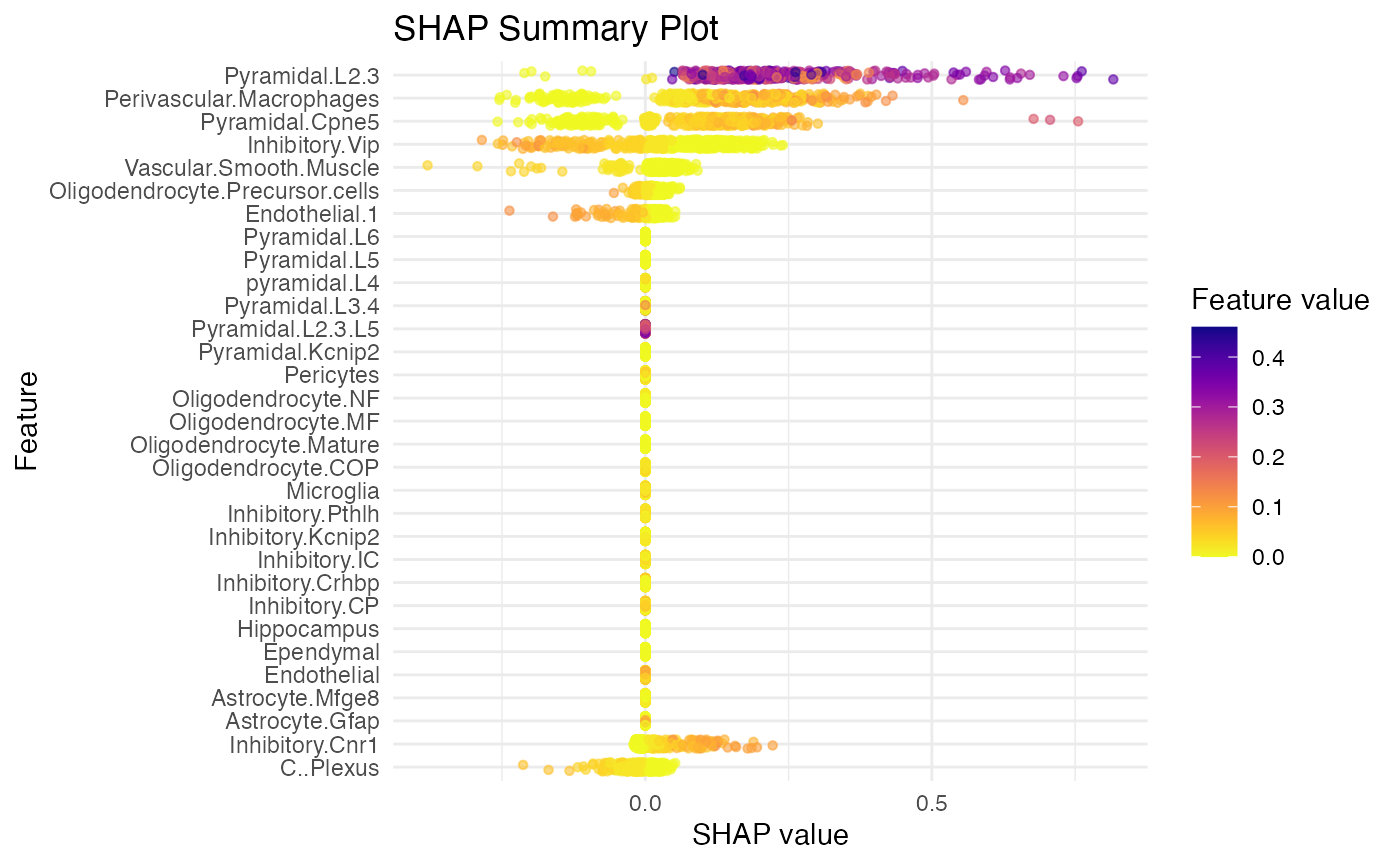

SHAP summary plot

SpaPheno_SHAP_summary_plot(shap_test_plus, top_n = 31)

SHAP residual analysis

resi_result <- SpaPheno_SHAP_residual_analysis(
  shap_df = shap_test_plus,
  feature_name = "Perivascular.Macrophages",
  coordinate_df = test_coordinate, size = 0.8
)
resi_hot <- resi_result$residual_table
head(resi_hot[order(abs(resi_hot$phi_resid_z), decreasing = T), ], 5)

##                      feature        phi   phi.var feature.value    sample
## 420 Perivascular.Macrophages  0.3887959 0.2184542          0.06 cell_5612
## 483 Perivascular.Macrophages -0.2546234 0.1502212          0.00 cell_4530
## 493 Perivascular.Macrophages -0.2535509 0.1451300          0.00 cell_4650
## 457 Perivascular.Macrophages  0.5548111 0.2055735          0.12 cell_5593
## 39  Perivascular.Macrophages  0.3240469 0.1976987          0.04 cell_5790
##     phi_residual phi_resid_z   resid_group color_group
## 420    0.2360473    2.642347 High residual        High
## 483   -0.2356644   -2.638060  Low residual         Low
## 493   -0.2345918   -2.626054  Low residual         Low
## 457    0.2303550    2.578626 High residual        High
## 39     0.2285343    2.558245 High residual        High

SpaPheno_SHAP_waterfall_plot(shap_test_plus, "cell_5593", top_n = 10)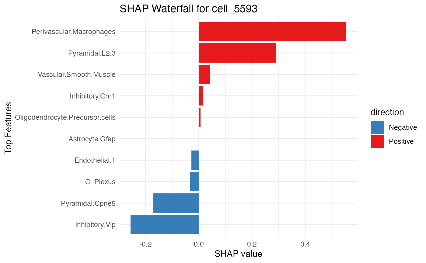

resi_result$dependence_plot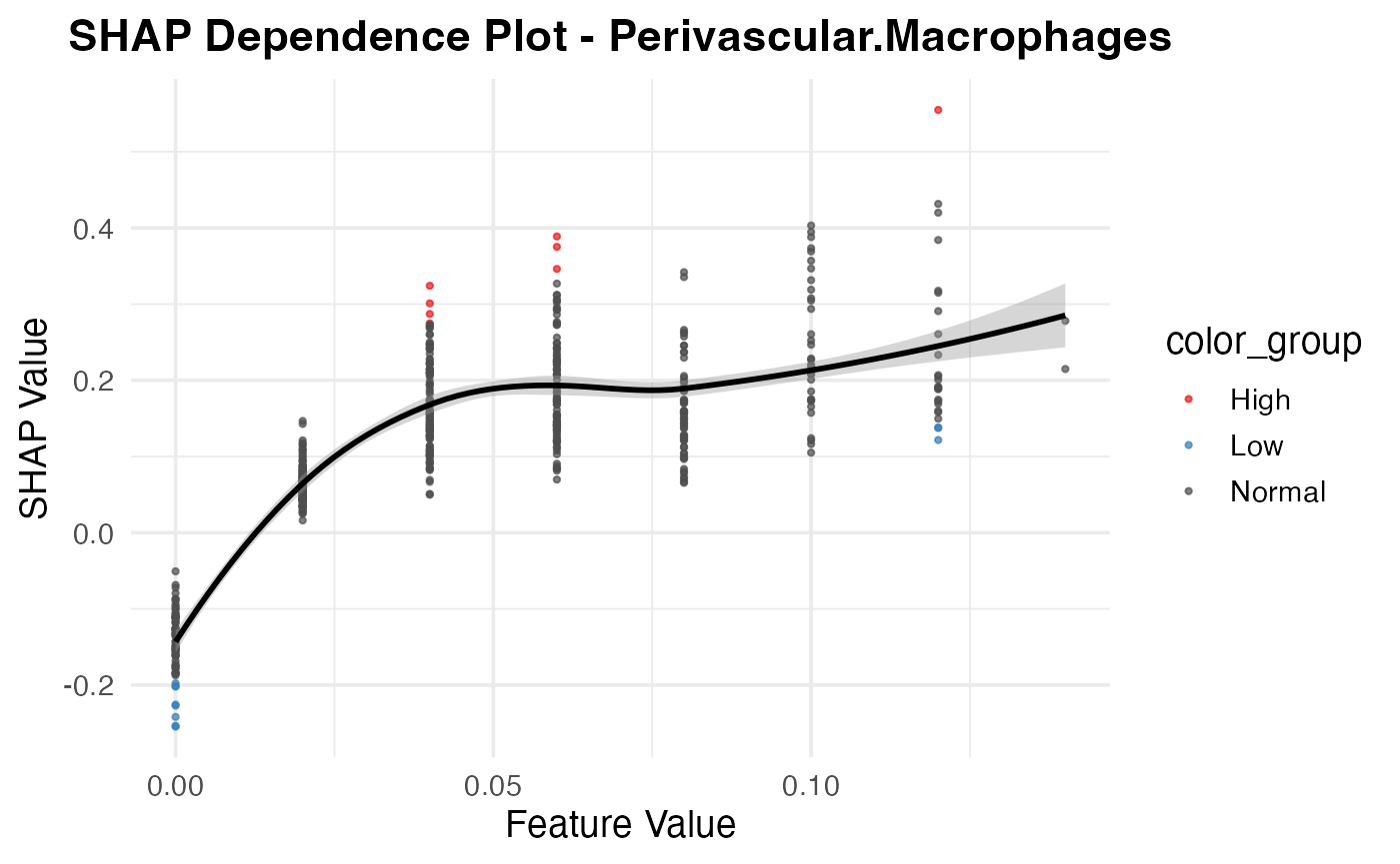

resi_result$spatial_plot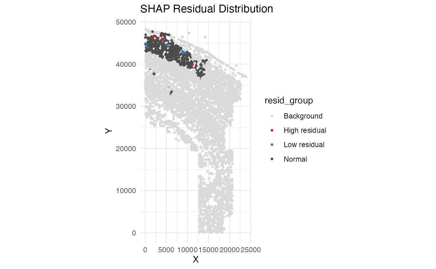

Simulation STARmap

load data

rm(list = ls())

load(system.file("extdata", "Simulation_STARmap.RData", package = "SpaPheno"))

ggplot(test_coordinate, aes(x = X, y = Y, color = sample_information_cellType)) +
  geom_point()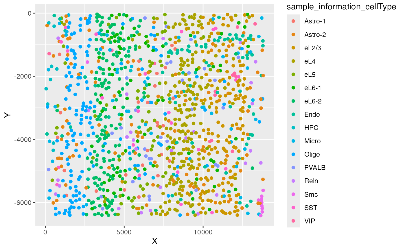

ggplot(test_coordinate, aes(x = X, y = Y, color = sample_information_region)) +
  geom_point()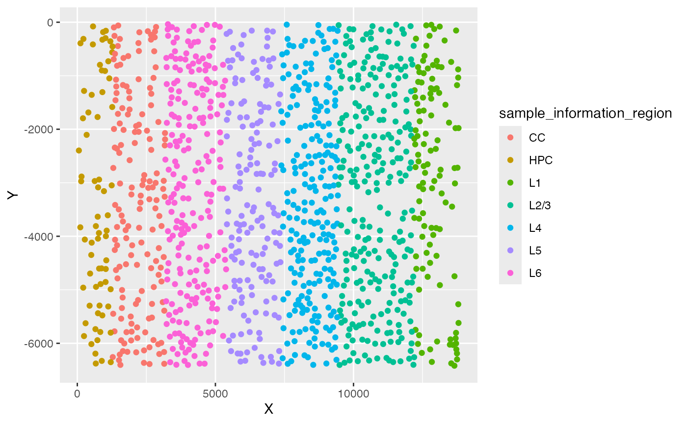

Choose simulated phenotypes

region_all <- names(table(sample_information_region))
phenotype_simu <- region_all[c(2, 6)]
sample_information_region_choose <- sample_information_region
sample_information_region_choose[!sample_information_region_choose %in% phenotype_simu] <- NA

Ground truth of simulated phenotypes

custom_colors <- c("red", "lightgray", "blue")
names(custom_colors) <- c(phenotype_simu[2], "Background", phenotype_simu[1])
sample_information_region_choose[!sample_information_region_choose %in% phenotype_simu] <- "Background"
Ground_truth <- factor(sample_information_region_choose[row.names(test_coordinate)], 
                       levels = c(phenotype_simu[1], "Background", phenotype_simu[2]))
ggplot(test_coordinate, aes(x = X, y = Y, color = Ground_truth)) +
  geom_point(size = 1) +
  scale_color_manual(values = custom_colors)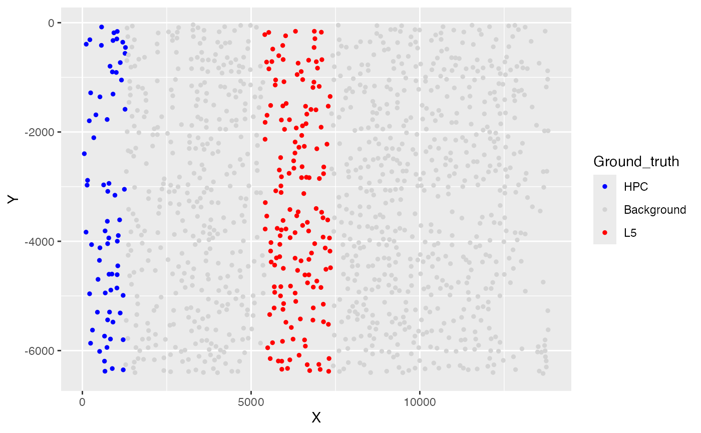

Obtain simulated data with phenotypes

pseudo_bulk_simi <- generate_simulated_bulk_data(
  input_data = sample_information_cellType, 
  region_labels = sample_information_region, 
  phenotypes = phenotype_simu, 
  perturbation_percent = 0.1, 
  num_samples = 50,
  mode = "proportion")

pseudo_bulk_df1 <- pseudo_bulk_simi[[1]]
pseudo_bulk_df2 <- pseudo_bulk_simi[[2]]

bulk_decon <- as.matrix(cbind(pseudo_bulk_df1, pseudo_bulk_df2))
bulk_decon <- t(apply(bulk_decon, 2, function(x) {
  x / sum(x)
}))
bulk_pheno <- rep(c(0, 1), each = 50)
names(bulk_pheno) <- c(colnames(pseudo_bulk_df1), colnames(pseudo_bulk_df2))
family <- "binomial"

Obtain prediction results

PhenoResult <- SpatialPhenoMap(
  bulk_decon = bulk_decon,
  bulk_pheno = bulk_pheno, 
  family = family, 
  coord = test_coordinate, 
  resolution = "single_cell", 
  sample_information_cellType = sample_information_cellType, 
  n_perm = 1, 
  p = 0.001
)

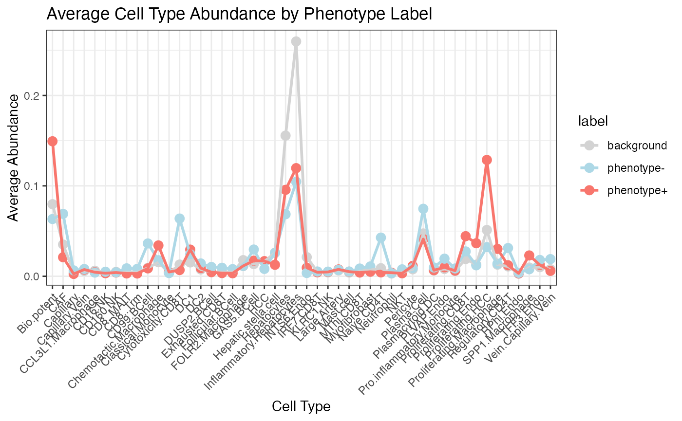
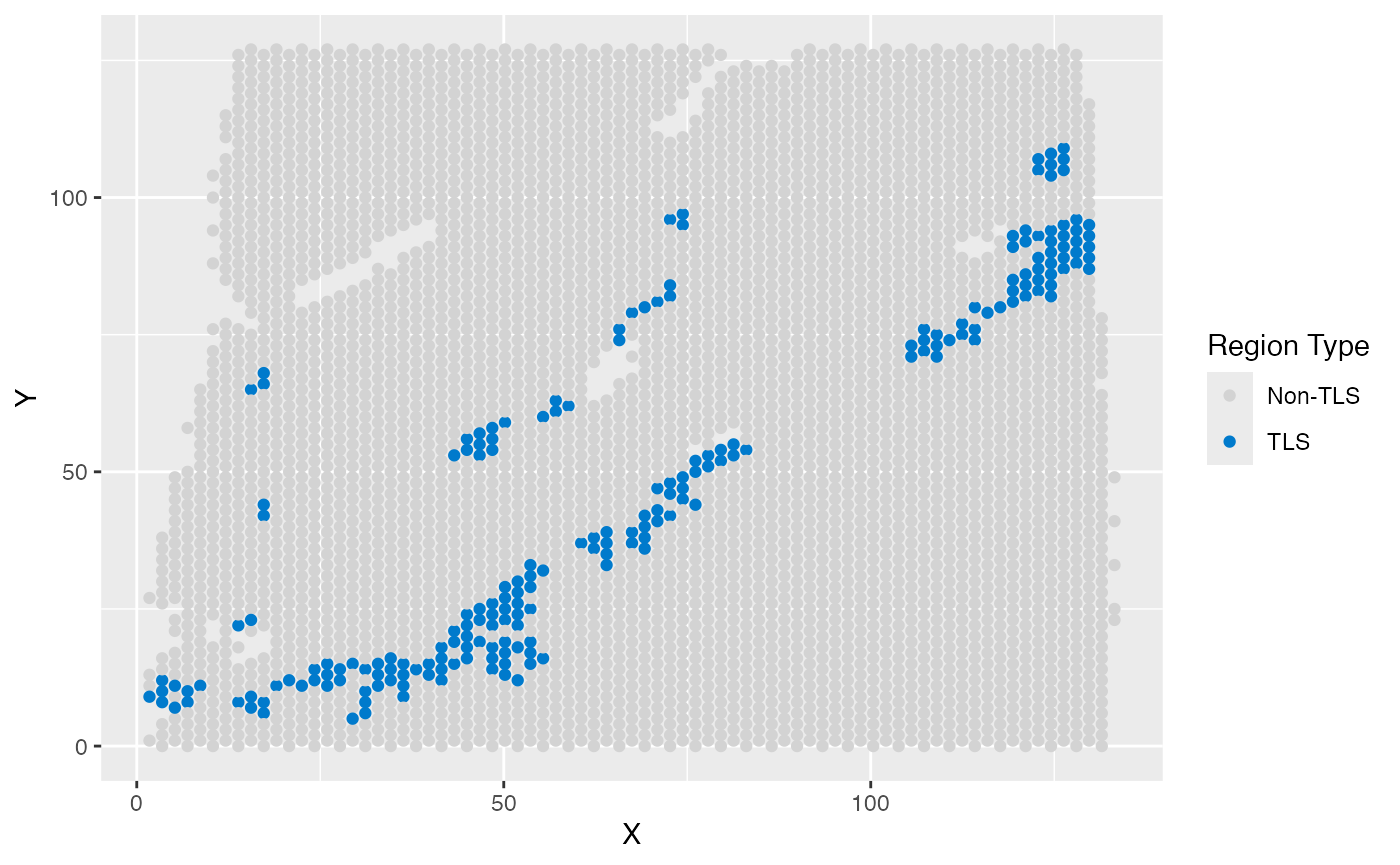
Survival HCC

load demo data

rm(list = ls())

load(system.file("extdata", "HCC_survival.RData", package = "SpaPheno"))

### TLS label
ggplot(test_coordinate, aes(x = X, y = Y, color = sample_information_region)) +
  geom_point(size = 1.5) +
  scale_color_manual(
    values = c(
      "TLS" = "#007ACC",   
      "nonTLS" = "lightgray" 
    ),
    name = "Region Type", 
    labels = c("Non-TLS", "TLS")
  )

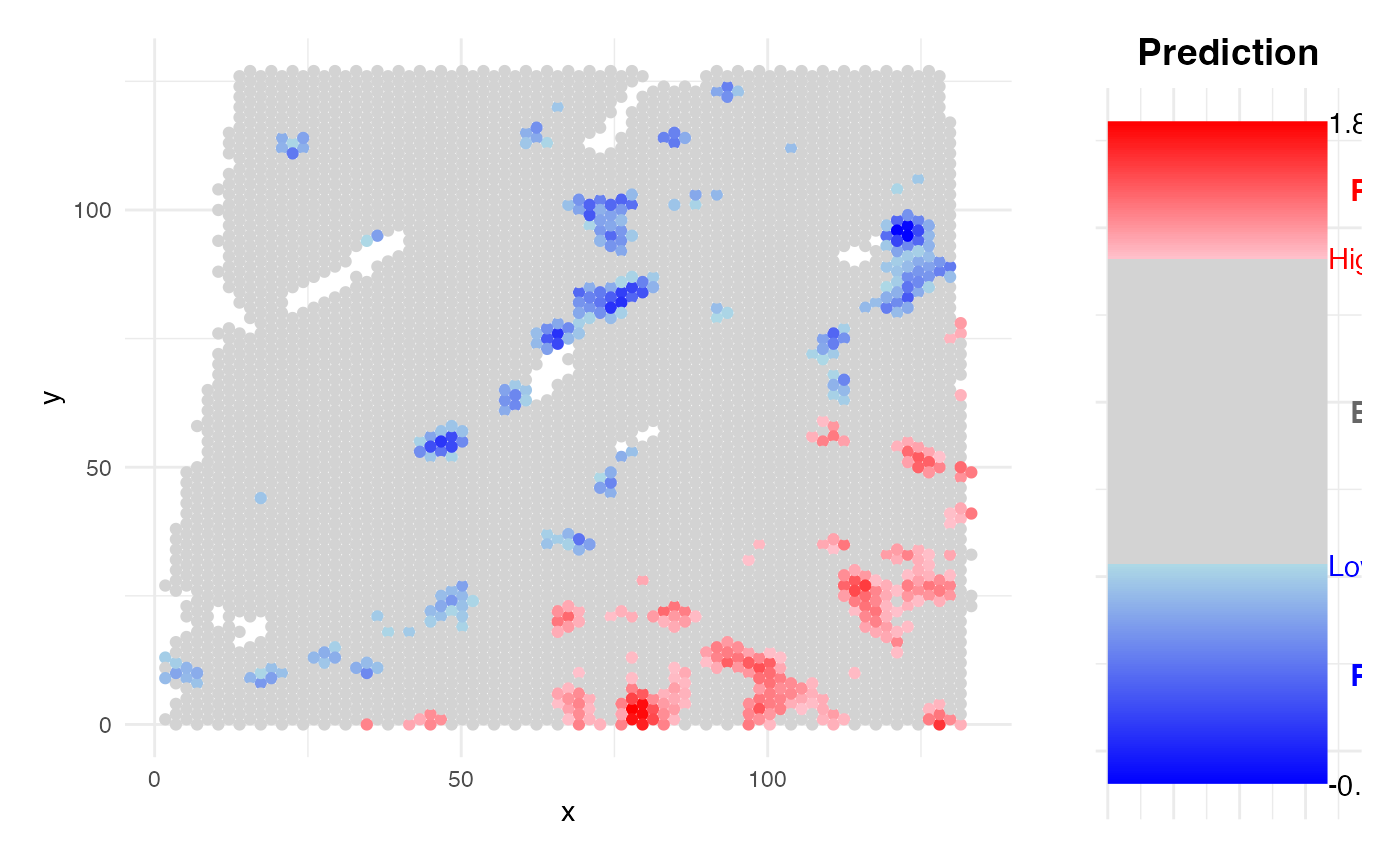
Obtain prediction results

PhenoResult <- SpatialPhenoMap(
  bulk_decon = bulk_decon,
  bulk_pheno = bulk_pheno,
  family = "cox",
  coord = test_coordinate,
  resolution = "spot",
  sample_information_decon = ST_decon,
  size = 1.5,
  n_perm = 1,
  p = 0.001,
  r = 4
)

SHAP analysis

pred_result <- PhenoResult$pred_score
phenoPlus <- row.names(pred_result[pred_result$label %in% "phenotype+", ])
phenoMinus <- row.names(pred_result[pred_result$label %in% "phenotype-", ])

model <- PhenoResult$model
X <- PhenoResult$cell_type_distribution[phenoMinus, ]
shap_test <- compute_shap_spatial(model, bulk_decon, bulk_pheno, X)
head(shap_test)

##             feature           phi      phi.var feature.value             sample
## 1        Bio.potent  0.0005838659 1.551781e-05   0.105472520 AAACAAGTATCTCCCA-1
## 2               CAF -0.0435152693 1.767573e-03   0.119948046 AAACAAGTATCTCCCA-1
## 3 CCL3L1.Macrophage  0.0000000000 0.000000e+00   0.005836406 AAACAAGTATCTCCCA-1
## 4         CD8..MAIT -0.0197043006 3.004776e-04   0.009533719 AAACAAGTATCTCCCA-1
## 5          CD8..Trm -0.0520022782 2.085855e-03   0.008196035 AAACAAGTATCTCCCA-1
## 6           CD16.NK  0.0500187685 3.619665e-03   0.006682971 AAACAAGTATCTCCCA-1

SpaPheno_SHAP_summary_plot(shap_test, top_n = 10)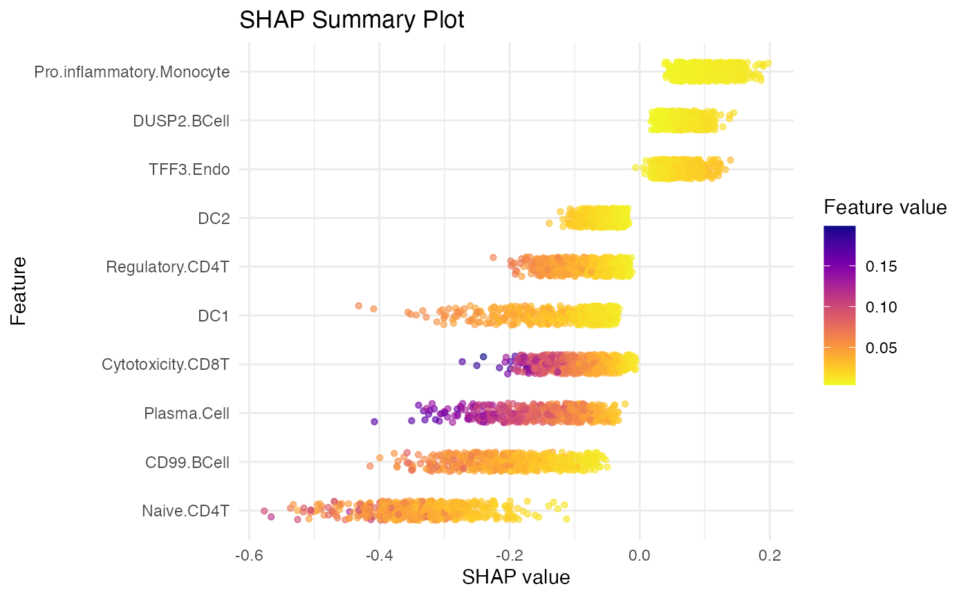

SHAP residual analysis

resi_result <- SpaPheno_SHAP_residual_analysis(
  shap_df = shap_test,
  feature_name = "Naive.CD4T",
  coordinate_df = test_coordinate, size = 0.8
)
resi_result$dependence_plot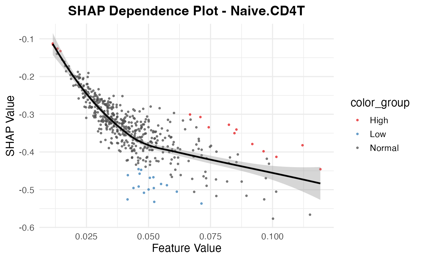

resi_result$spatial_plot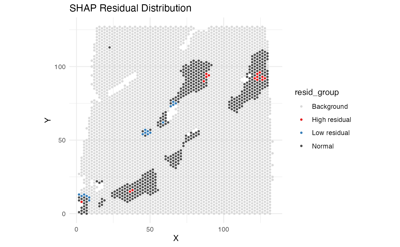

SHAP waterfall plot

resi_hot <- resi_result$residual_table
head(resi_hot[order(abs(resi_hot$phi_resid_z), decreasing = T), ], 10)

##        feature        phi    phi.var feature.value             sample
## 30  Naive.CD4T -0.5257900 0.13837004    0.04155390 AATTCCAACTTGGTGA-1
## 51  Naive.CD4T -0.3821739 0.07231961    0.11206579 ACGACTCTAGGGCCGA-1
## 474 Naive.CD4T -0.5322684 0.17930920    0.05231648 TTATATACGCTGTCAC-1
## 420 Naive.CD4T -0.4955256 0.07926515    0.04394551 TCGCCTCGACCTGTTG-1
## 453 Naive.CD4T -0.5082004 0.09662787    0.04816872 TGGACTGTTCGCTCAA-1
## 181 Naive.CD4T -0.4916031 0.07350465    0.04604062 CGCATTAGCTAATAGG-1
## 331 Naive.CD4T -0.4994501 0.11421113    0.05003514 GTACTAAGATTTGGAG-1
## 136 Naive.CD4T -0.4456933 0.12689195    0.11926253 CAGGGCTAACGAAACC-1
## 419 Naive.CD4T -0.3278083 0.07309902    0.08241027 TCGCCTCCTTCGGCTC-1
## 379 Naive.CD4T -0.3405043 0.08242797    0.08543729 TAGCAGATACTTAGGG-1
##     phi_residual phi_resid_z   resid_group color_group
## 30    -0.1972143   -3.930519  Low residual         Low
## 51     0.1790110    3.567723 High residual        High
## 474   -0.1681884   -3.352028  Low residual         Low
## 420   -0.1590603   -3.170102  Low residual         Low
## 453   -0.1578033   -3.145050  Low residual         Low
## 181   -0.1482263   -2.954179  Low residual         Low
## 331   -0.1428959   -2.847942  Low residual         Low
## 136    0.1392326    2.774932 High residual        High
## 419    0.1355471    2.701479 High residual        High
## 379    0.1328367    2.647461 High residual        High

SpaPheno_SHAP_waterfall_plot(shap_test, "TCGCCGGAGAGTCTTA-1", top_n = 48)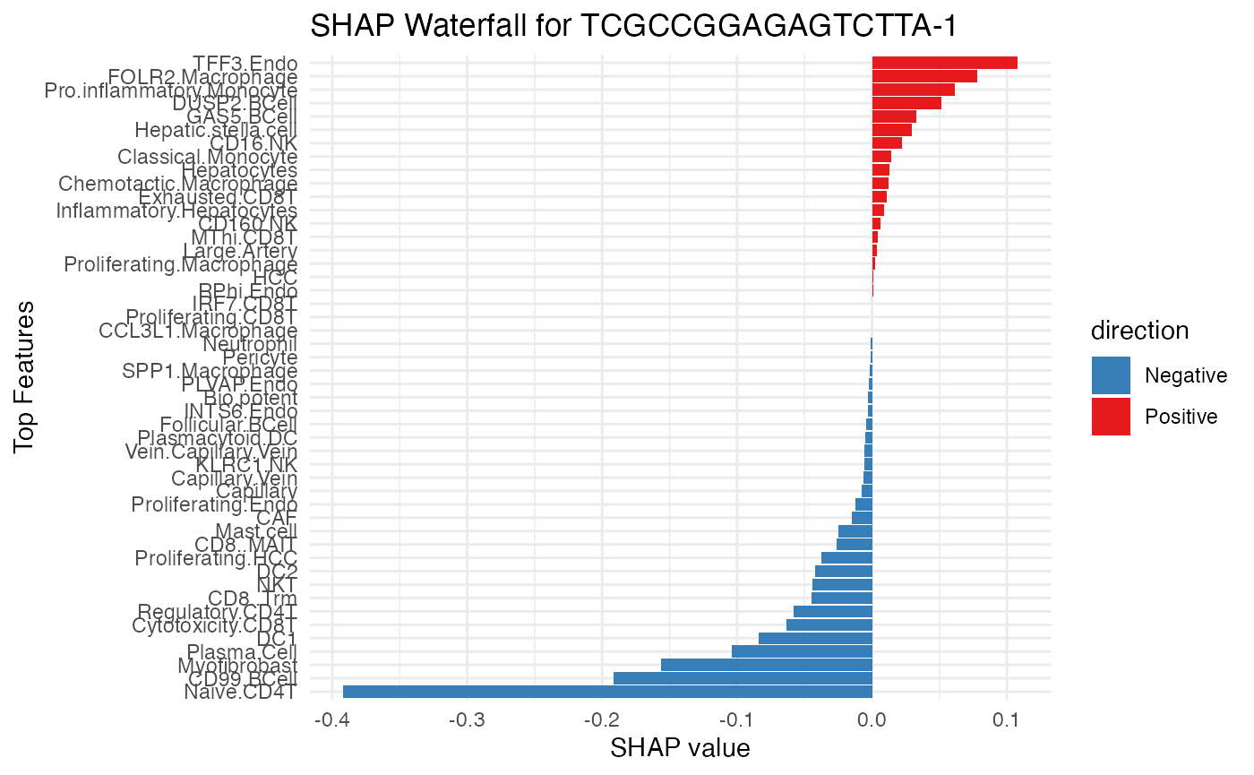

SHAP dependence plot

TCell_subtypes <- unique(shap_test$feature)[str_detect(unique(shap_test$feature), "CD.T")]
BCell_subtypes <- unique(shap_test$feature)[str_detect(unique(shap_test$feature), "BCell")]
Monocyte_subtypes <- unique(shap_test$feature)[str_detect(unique(shap_test$feature), "Monocyte")]
Macrophage_subtypes <- unique(shap_test$feature)[str_detect(unique(shap_test$feature), "Macrophage")]

SpaPheno_SHAP_dependence_plot(shap_test, TCell_subtypes)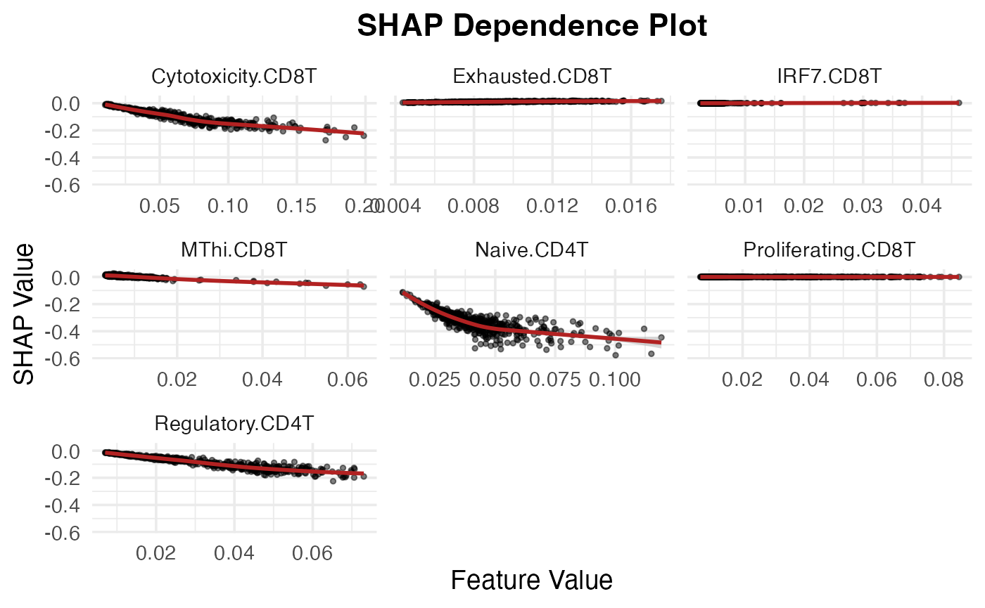

SpaPheno_SHAP_dependence_plot(shap_test, BCell_subtypes)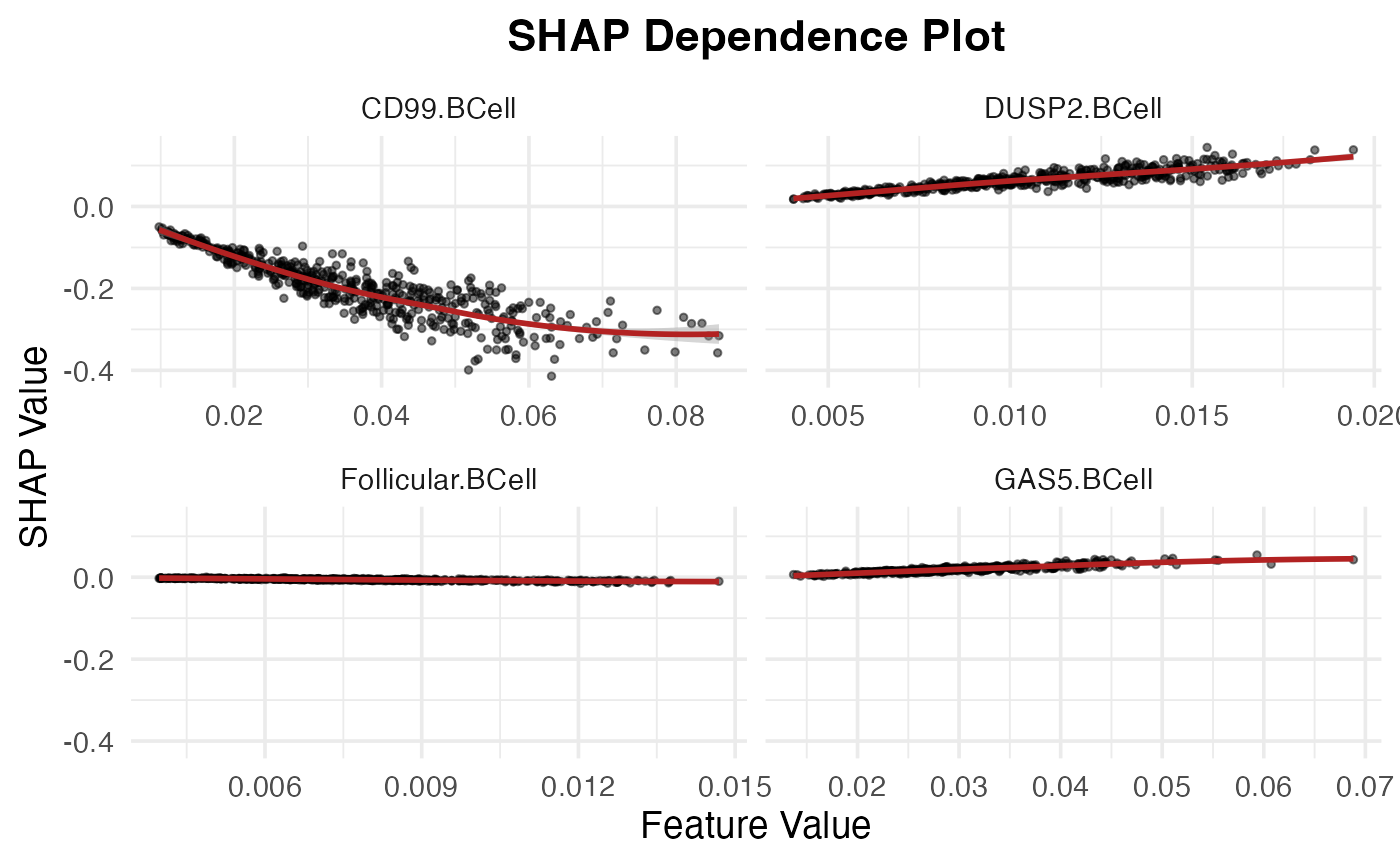

SpaPheno_SHAP_dependence_plot(shap_test, Monocyte_subtypes)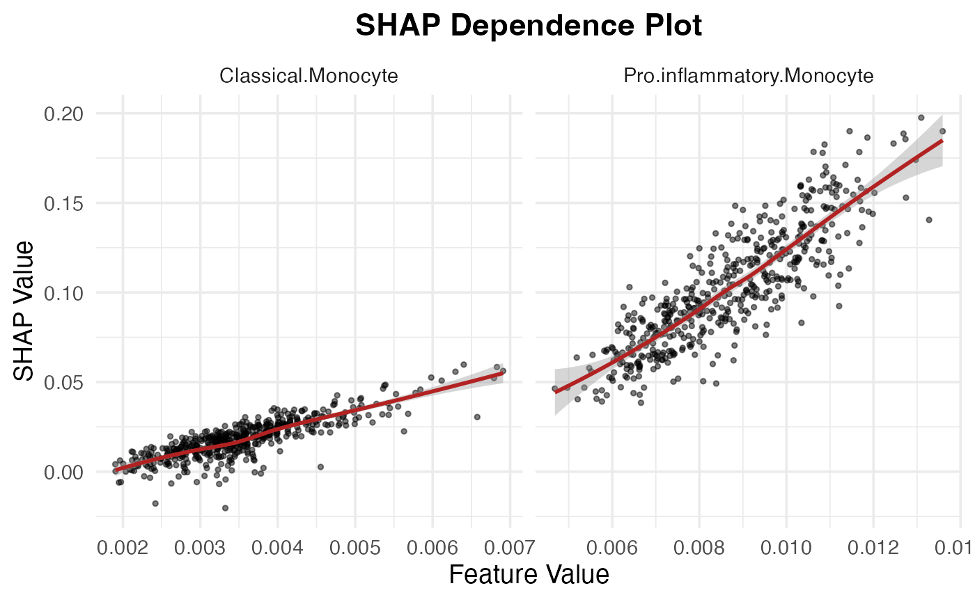

SpaPheno_SHAP_dependence_plot(shap_test, Macrophage_subtypes)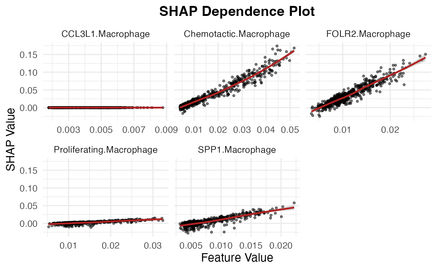

Survival BRCA

load demo data

rm(list = ls())

load("BRCAsurvival.RData")

### survival phenotype
TCGA_survival_each <- TCGA_BRCA$TCGA.BRCA.survival.tsv
Survival_TCGA_choose <- as.data.frame(TCGA_survival_each)
row.names(Survival_TCGA_choose) <- Survival_TCGA_choose[, 1]

### common samples between survival phenotype and deconvolution
sample_information_decon_TCGA_choose <- BRCA_decon[intersect(as.data.frame(TCGA_survival_each)[, 1], row.names(BRCA_decon)), ]
Survival_TCGA_choose <- Survival_TCGA_choose[row.names(sample_information_decon_TCGA_choose), ]

### survival object
surv_obj <- Surv(Survival_TCGA_choose$OS.time, Survival_TCGA_choose$OS)

### ST
test_coordinate <- as.data.frame(cbind(BRCA_ST$x, BRCA_ST$y))
colnames(test_coordinate) <- c("X", "Y")
sample_information_region <- BRCA_ST$label
bulk_decon <- sample_information_decon_TCGA_choose
bulk_pheno <- surv_obj
family <- "cox"

coord <- test_coordinate
resolution <- "spot"
colnames(bulk_decon) <- gsub("^[^_]*_[^_]*_[^_]*_sf_", "", colnames(bulk_decon))
colnames(sample_information_decon) <- gsub("^[^_]*_[^_]*_[^_]*_sf_", "", colnames(sample_information_decon))

Ground truth

ggplot(test_coordinate, aes(x = X, y = Y, color = sample_information_region)) +
  geom_point(size = 4)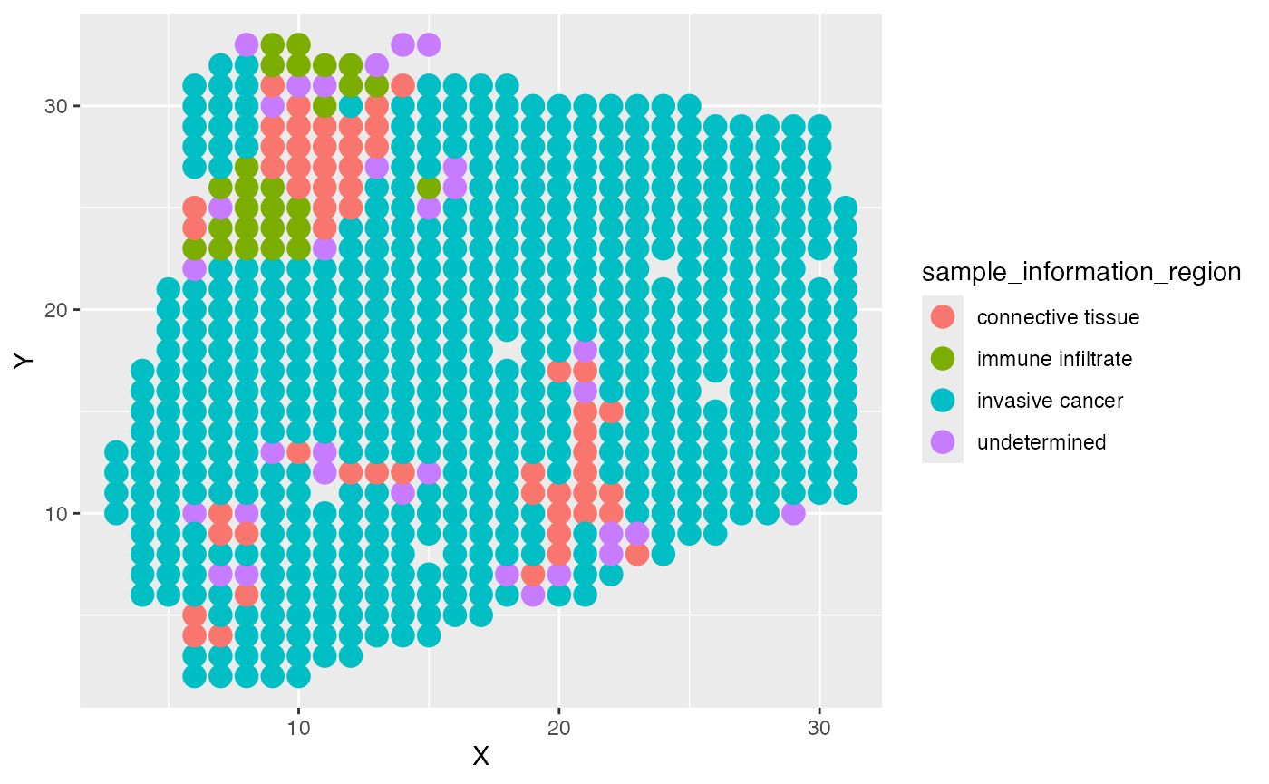

Obtain predicion results

PhenoResult <- SpatialPhenoMap(
  bulk_decon = bulk_decon, 
  bulk_pheno = bulk_pheno, 
  family = "cox", 
  coord = test_coordinate, 
  resolution = "spot", 
  sample_information_decon = sample_information_decon,
  size = 5, 
  n_perm = 1, 
  p = 0.001, 
  r = 2)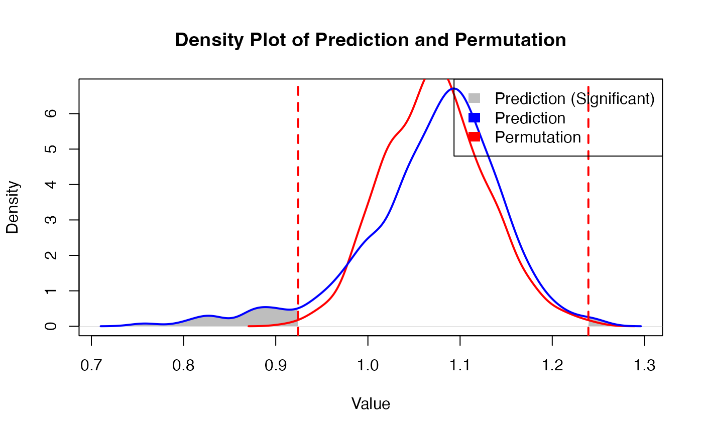

Survival KIRC

load demo data

rm(list = ls())

load("KIRC_survival.RData")

### survival phenotype
TCGA_survival_each <- TCGA_KIRC$TCGA.KIRC.survival.tsv
Survival_TCGA_choose <- as.data.frame(TCGA_survival_each)
row.names(Survival_TCGA_choose) <- Survival_TCGA_choose[, 1]

### common samples between survival phenotype and deconvolution
sample_information_decon_TCGA_choose <- KIRC_decon[intersect(as.data.frame(TCGA_survival_each)[, 1], row.names(KIRC_decon)), ]
Survival_TCGA_choose <- Survival_TCGA_choose[row.names(sample_information_decon_TCGA_choose), ]

### survival object
surv_obj <- Surv(Survival_TCGA_choose$OS.time, Survival_TCGA_choose$OS)

test_coordinate <- as.data.frame(cbind(KIRC_ST$x, KIRC_ST$y))
colnames(test_coordinate) <- c("X", "Y")
sample_information_region <- KIRC_ST$TLSanno
bulk_decon <- sample_information_decon_TCGA_choose
bulk_pheno <- surv_obj
family <- "cox"

coord <- test_coordinate
resolution <- "spot"
colnames(bulk_decon) <- gsub("^[^_]*_[^_]*_[^_]*_sf_", "", colnames(bulk_decon))
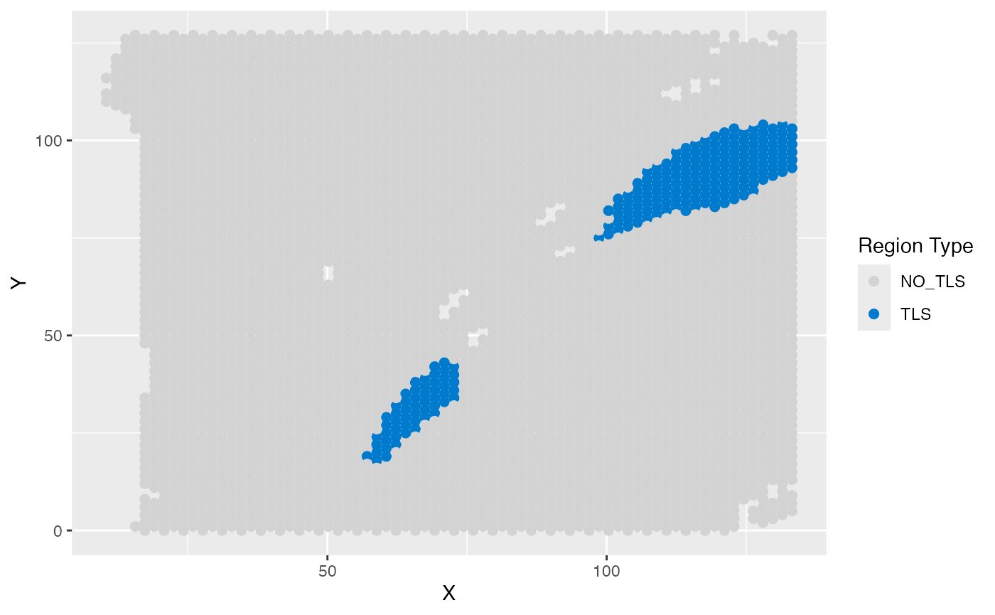
colnames(sample_information_decon) <- gsub("^[^_]*_[^_]*_[^_]*_sf_", "", colnames(sample_information_decon))

Ground Truth

ggplot(test_coordinate, aes(x = X, y = Y, color = sample_information_region)) +
  geom_point(size = 2) +
  scale_color_manual(
    values = c(
      "TLS" = "#007ACC",
      "NO_TLS" = "lightgray"
    ),
    name = "Region Type",
    labels = c("NO_TLS", "TLS")
  )

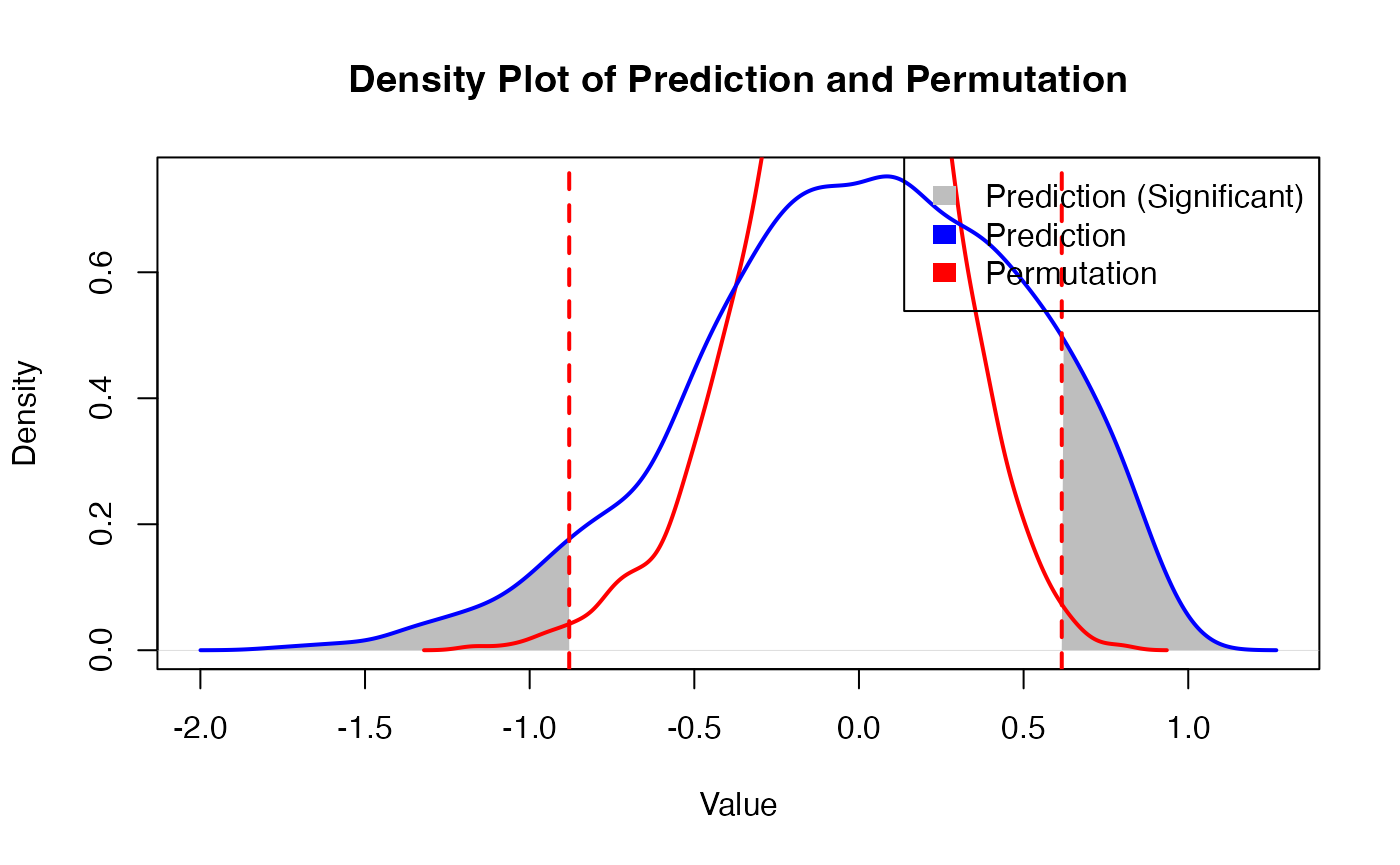
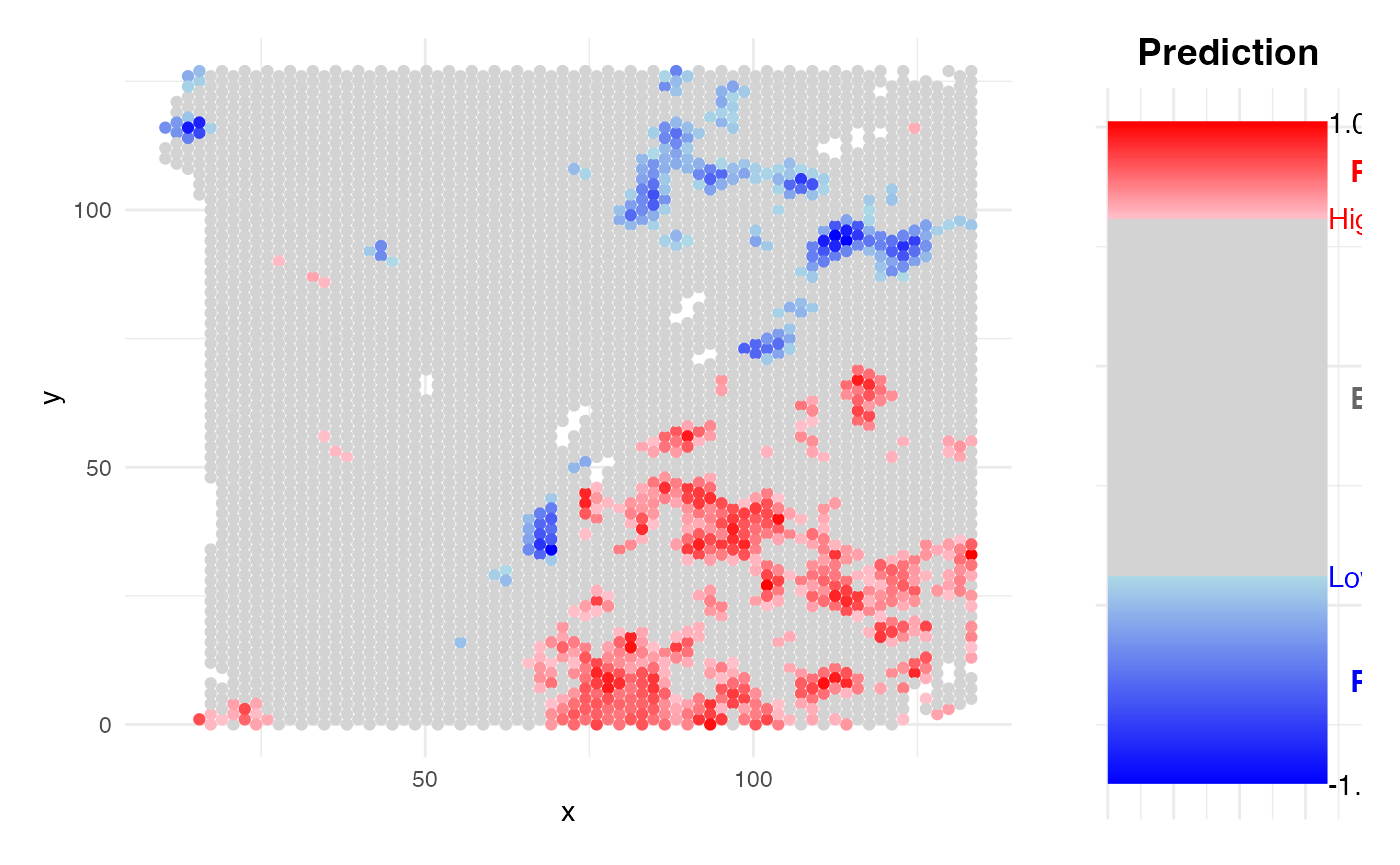
Prediction result

PhenoResult <- SpatialPhenoMap(
  bulk_decon = bulk_decon,
  bulk_pheno = bulk_pheno, 
  family = family, 
  coord = test_coordinate, 
  resolution = "spot", 
  sample_information_decon = sample_information_decon, 
  size = 1.5, 
  n_perm = 1, 
  p = 0.005, 
  r = 2
)

Hclust of low risk region

PhenotypeHclust(PhenoResult, "phenotype-", test_coordinate, size = 1.5)

Stage HCC

load data

rm(list = ls())
load("HCC_stage.RData")

#### common samples between stage phenotype and deconvolution
common_sample <- intersect(names(sample_information_stage), row.names(LIHC_decon))
LIHC_decon <- LIHC_decon[common_sample, ]
sample_information_stage <- sample_information_stage[common_sample]


sample_information_region <- HCC_ST$TLSanno
test_coordinate <- HCC_ST@meta.data[, 4:5]
colnames(test_coordinate) <- c("X", "Y")

bulk_decon <- LIHC_decon
bulk_pheno <- sample_information_stage
family <- "gaussian"

coord <- test_coordinate
resolution <- "spot"
sample_information_decon <- sample_information_decon

colnames(bulk_decon) <- gsub("^[^_]*_[^_]*_[^_]*_sf_", "", colnames(bulk_decon))
colnames(sample_information_decon) <- gsub("^[^_]*_[^_]*_[^_]*_sf_", "", colnames(sample_information_decon))

### TLS label
ggplot(test_coordinate, aes(x = X, y = Y, color = sample_information_region)) +
  geom_point(size = 1.5) +
  scale_color_manual(
    values = c(
      "TLS" = "#007ACC", 
      "nonTLS" = "lightgray" 
    ),
    name = "Region Type",
    labels = c("Non-TLS", "TLS")
  )

Obtain prdiction result

PhenoResult <- SpatialPhenoMap(
  bulk_decon = bulk_decon,
  bulk_pheno = bulk_pheno,
  family = family,
  coord = test_coordinate,
  resolution = "spot", 
  sample_information_decon = sample_information_decon, 
  size = 1.5, 
  n_perm = 1, 
  p = 0.001
)

ICB melanoma

load data

rm(list = ls())
load("Melanoma_ICB.RData")

test_coordinate <- head(Melanoma_ST, length(Melanoma_ST$x))[, 4:5]
colnames(test_coordinate) <- c("Y", "X")
test_coordinate <- test_coordinate[, c("X", "Y")]

bulk_decon <- bulk_decon
bulk_pheno <- bulk_pheno
family <- "binomial"

coord <- test_coordinate
resolution <- "spot"
sample_information_decon <- Melanoma_ST_decon
# sample_information_decon<-t(apply(sample_information_decon,1,function(x){x/sum(x)}))
colnames(bulk_decon) <- gsub("^[^_]*_[^_]*_[^_]*_sf_", "", colnames(bulk_decon))
colnames(sample_information_decon) <- gsub("^[^_]*_[^_]*_[^_]*_sf_", "", colnames(sample_information_decon))

Obtain predicion results

PhenoResult <- SpatialPhenoMap(
  bulk_decon = bulk_decon, 
  bulk_pheno = bulk_pheno, 
  family = family, 
  coord = test_coordinate, 
  resolution = "spot", 
  sample_information_decon = sample_information_decon, 
  size = 5,
  n_perm = 1,
  p = 0.01)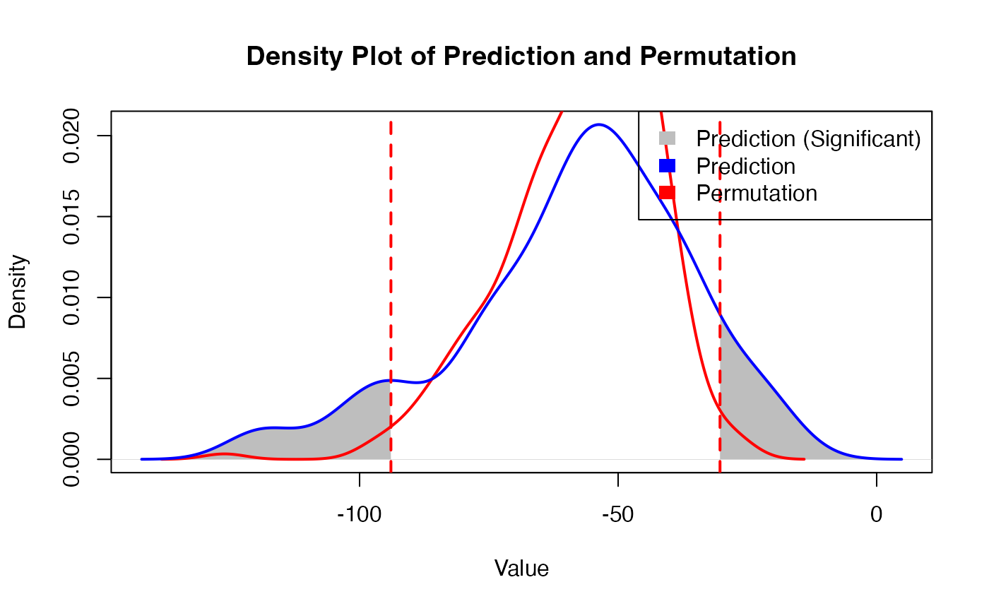

Summary

This tutorial provides a step-by-step demonstration of how to apply the SpaPheno R package to predict and interpret spatially informed phenotypes using spatial transcriptomic and bulk-like simulated data.

Across multiple datasets and biological contexts—including simulated osmFISH and STARmap, and real-world HCC, BRCA, and KIRC samples—this guide illustrates the core capabilities of SpaPheno:

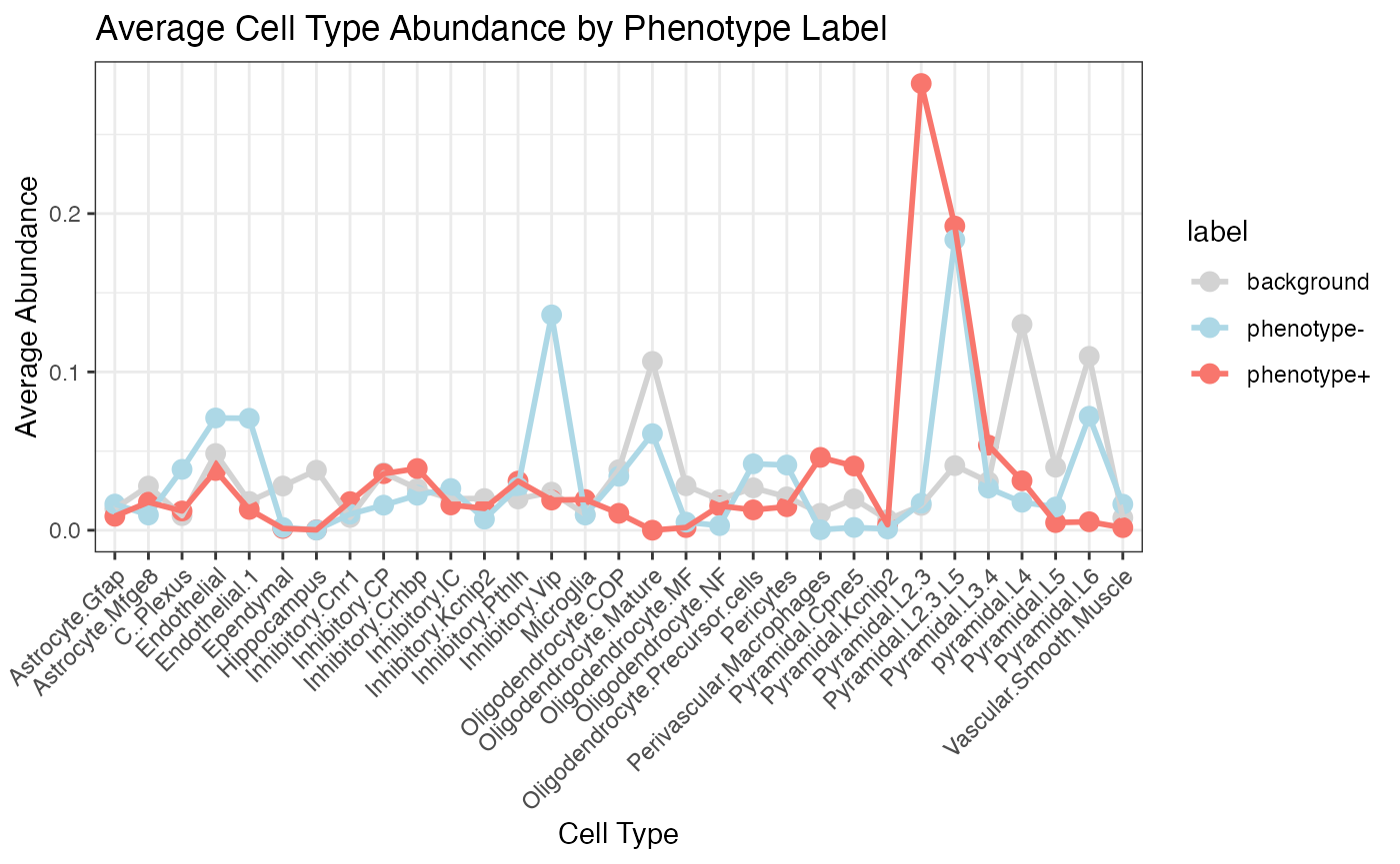
Phenotype Simulation: It shows how to simulate bulk-like phenotypic data from spatial single-cell annotations, capturing cell-type composition per region.
Model Building: Using a logistic, linear, or Cox proportional hazards model with automated alpha selection, SpaPheno learns a predictive model from bulk deconvolution data and phenotypic labels.
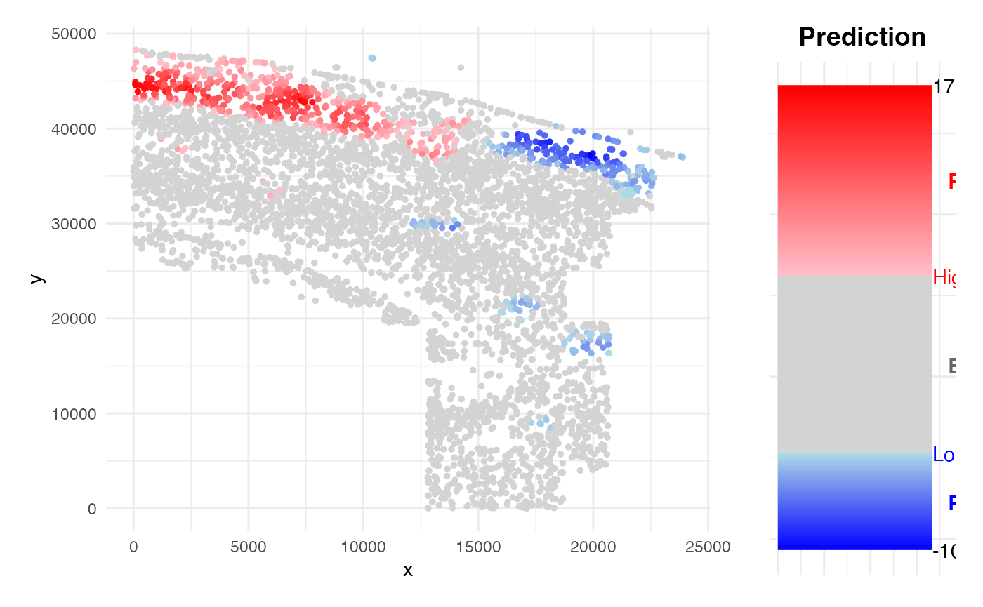
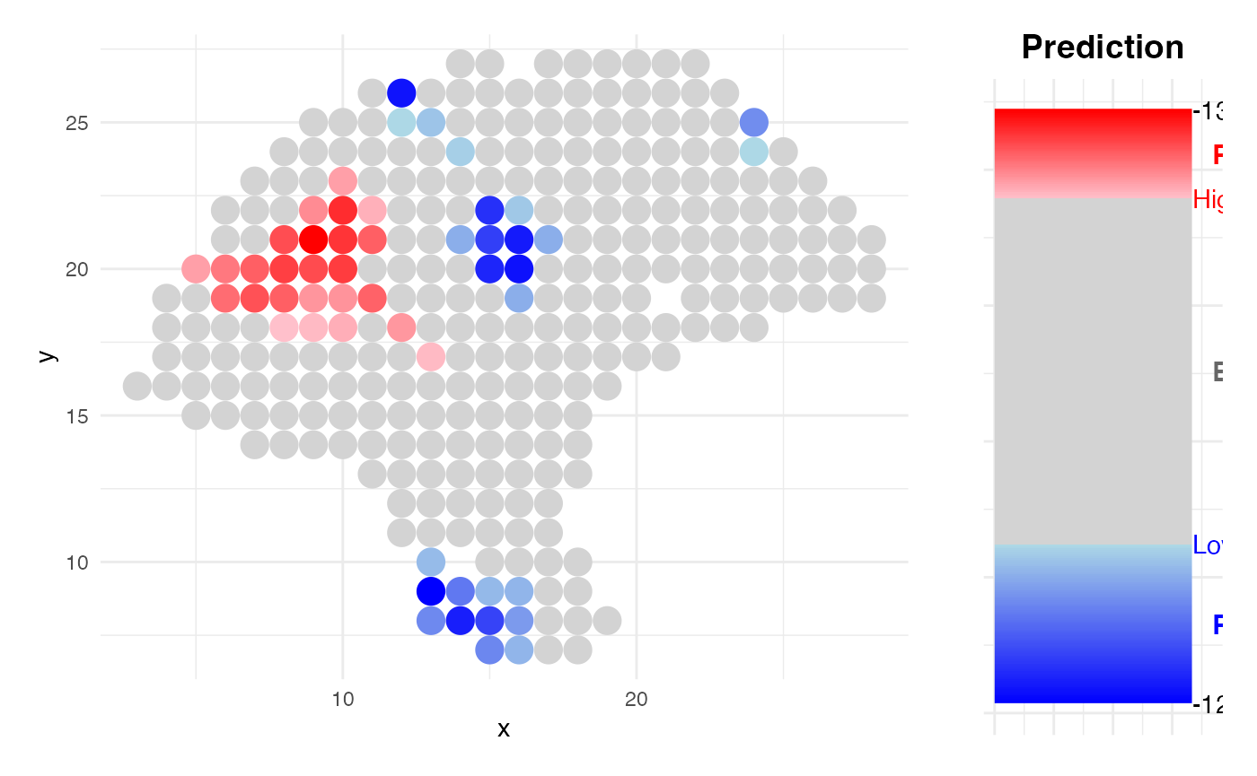
Spatial Prediction: The model is applied back to spatial neighborhoods (either at spot or single-cell resolution) to estimate and visualize spatial risk distributions.
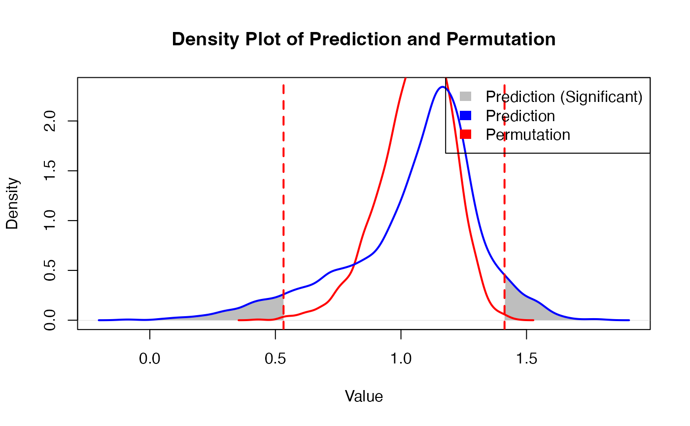
Permutation Testing: The tool quantifies the significance of spatial predictions using randomized coordinate-based permutation testing.
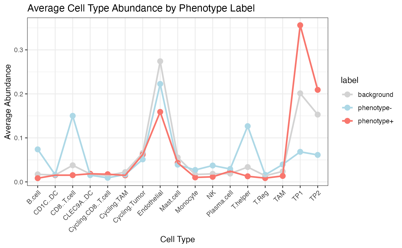
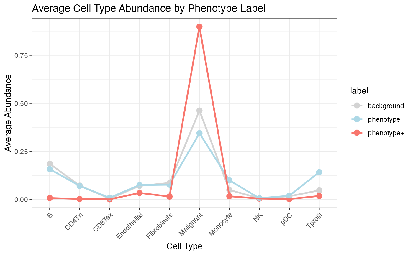
SHAP-based Interpretation: By leveraging SHAP (SHapley Additive exPlanations), SpaPheno identifies the most important cell types contributing to spatial phenotype risk, at both population and single-cell levels.
Residual & Dependence Analysis: SpaPheno offers residual maps and dependence plots to explore non-modeled effects and spatial patterns, enhancing interpretability.

In essence, SpaPheno bridges spatial cellular architecture and clinical or experimental phenotypes, enabling researchers to map spatial risk, decode key microenvironmental drivers, and explore the mechanistic underpinnings of tissue-level phenotypes.

This reproducible tutorial serves as a valuable resource for both method developers and biological researchers aiming to explore the spatial origins of complex phenotypes.

System information

sessionInfo()

## R version 4.4.3 (2025-02-28)
## Platform: aarch64-apple-darwin20
## Running under: macOS Sequoia 15.6.1
## 
## Matrix products: default
## BLAS:   /Library/Frameworks/R.framework/Versions/4.4-arm64/Resources/lib/libRblas.0.dylib 
## LAPACK: /Library/Frameworks/R.framework/Versions/4.4-arm64/Resources/lib/libRlapack.dylib;  LAPACK version 3.12.0
## 
## locale:
## [1] en_US.UTF-8/en_US.UTF-8/en_US.UTF-8/C/en_US.UTF-8/en_US.UTF-8
## 
## time zone: Asia/Shanghai
## tzcode source: internal
## 
## attached base packages:
## [1] stats     graphics  grDevices utils     datasets  methods   base     
## 
## other attached packages:
##  [1] umap_0.2.10.0       fastcluster_1.3.0   philentropy_0.10.0 
##  [4] Seurat_5.3.1        SeuratObject_5.2.0  sp_2.2-0           
##  [7] survival_3.8-3      reshape2_1.4.4      lubridate_1.9.4    
## [10] forcats_1.0.1       stringr_1.6.0       dplyr_1.1.4        
## [13] purrr_1.2.0         readr_2.1.5         tidyr_1.3.1        
## [16] tibble_3.3.0        ggplot2_4.0.0       tidyverse_2.0.0    
## [19] SpaPheno_0.0.2      BiocManager_1.30.26 BiocStyle_2.34.0   
## 
## loaded via a namespace (and not attached):
##   [1] RcppAnnoy_0.0.22       splines_4.4.3          later_1.4.4           
##   [4] polyclip_1.10-7        hardhat_1.4.2          pROC_1.19.0.1         
##   [7] rpart_4.1.24           fastDummies_1.7.5      lifecycle_1.0.4       
##  [10] globals_0.18.0         lattice_0.22-7         MASS_7.3-65           
##  [13] backports_1.5.0        magrittr_2.0.4         plotly_4.11.0         
##  [16] sass_0.4.10            rmarkdown_2.30         jquerylib_0.1.4       
##  [19] yaml_2.3.10            httpuv_1.6.16          otel_0.2.0            
##  [22] sctransform_0.4.2      askpass_1.2.1          spam_2.11-1           
##  [25] spatstat.sparse_3.1-0  reticulate_1.44.0      cowplot_1.2.0         
##  [28] pbapply_1.7-4          RColorBrewer_1.1-3     abind_1.4-8           
##  [31] Rtsne_0.17             Metrics_0.1.4          nnet_7.3-20           
##  [34] ipred_0.9-15           lava_1.8.2             ggrepel_0.9.6         
##  [37] irlba_2.3.5.1          listenv_0.10.0         spatstat.utils_3.2-0  
##  [40] goftest_1.2-3          RSpectra_0.16-2        spatstat.random_3.4-2 
##  [43] fitdistrplus_1.2-4     parallelly_1.45.1      pkgdown_2.1.3         
##  [46] codetools_0.2-20       tidyselect_1.2.1       shape_1.4.6.1         
##  [49] farver_2.1.2           viridis_0.6.5          matrixStats_1.5.0     
##  [52] stats4_4.4.3           spatstat.explore_3.5-3 jsonlite_2.0.0        
##  [55] caret_7.0-1            progressr_0.17.0       ggridges_0.5.7        
##  [58] iterators_1.0.14       systemfonts_1.3.1      foreach_1.5.2         
##  [61] tools_4.4.3            ragg_1.5.0             ica_1.0-3             
##  [64] Rcpp_1.1.0             glue_1.8.0             prodlim_2025.04.28    
##  [67] gridExtra_2.3          xfun_0.54              mgcv_1.9-3            
##  [70] withr_3.0.2            fastmap_1.2.0          iml_0.11.4            
##  [73] openssl_2.3.4          digest_0.6.37          timechange_0.3.0      
##  [76] R6_2.6.1               mime_0.13              textshaping_1.0.4     
##  [79] scattermore_1.2        tensor_1.5.1           dichromat_2.0-0.1     
##  [82] spatstat.data_3.1-9    generics_0.1.4         data.table_1.17.8     
##  [85] recipes_1.3.1          FNN_1.1.4.1            class_7.3-23          
##  [88] httr_1.4.7             htmlwidgets_1.6.4      uwot_0.2.3            
##  [91] ModelMetrics_1.2.2.2   pkgconfig_2.0.3        gtable_0.3.6          
##  [94] timeDate_4051.111      lmtest_0.9-40          S7_0.2.0              
##  [97] htmltools_0.5.8.1      dotCall64_1.2          bookdown_0.45         
## [100] scales_1.4.0           png_0.1-8              gower_1.0.2           
## [103] spatstat.univar_3.1-4  knitr_1.50             rstudioapi_0.17.1     
## [106] tzdb_0.5.0             checkmate_2.3.3        nlme_3.1-168          
## [109] cachem_1.1.0           zoo_1.8-14             SpaDo_1.2.0           
## [112] KernSmooth_2.23-26     parallel_4.4.3         miniUI_0.1.2          
## [115] desc_1.4.3             pillar_1.11.1          grid_4.4.3            
## [118] vctrs_0.6.5            RANN_2.6.2             promises_1.5.0        
## [121] xtable_1.8-4           cluster_2.1.8.1        evaluate_1.0.5        
## [124] cli_3.6.5              compiler_4.4.3         rlang_1.1.6           
## [127] future.apply_1.20.0    labeling_0.4.3         plyr_1.8.9            
## [130] fs_1.6.6               stringi_1.8.7          viridisLite_0.4.2     
## [133] deldir_2.0-4           lazyeval_0.2.2         spatstat.geom_3.6-0   
## [136] glmnet_4.1-10          Matrix_1.7-4           RcppHNSW_0.6.0        
## [139] hms_1.1.4              patchwork_1.3.2        future_1.67.0         
## [142] shiny_1.11.1           ROCR_1.0-11            igraph_2.2.1          
## [145] RcppParallel_5.1.11-1  bslib_0.9.0

Bin Duan

2026-04-17

Introduction

Installation

Data availability

Deconvolution Strategy

Parameter Selection for cell2location

1. N_cells_per_location

2. detection_alpha

Practical Recommendations

Simulation osmFISH

load data

Choose simulated phenotypes

Ground truth of simulated phenotypes

Simulating bulk data with phenotypes

Obtaining prediction results

SHAP analysis

SHAP summary plot

SHAP residual analysis

Simulation STARmap

load data

Choose simulated phenotypes

Ground truth of simulated phenotypes

Obtain simulated data with phenotypes

Obtain prediction results

Survival HCC

load demo data

Obtain prediction results

SHAP analysis

SHAP residual analysis

SHAP waterfall plot

SHAP dependence plot

Survival BRCA

load demo data

Ground truth

Obtain predicion results

Survival KIRC

load demo data

Ground Truth

Prediction result

Hclust of low risk region

Stage HCC

load data

Obtain prdiction result

ICB melanoma

load data

Obtain predicion results

Summary

System information